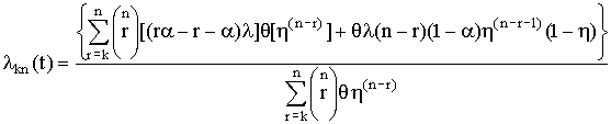
System failure rate in general terms. Failure rate - dependence of failure rate on time (product life curve). MTBF

Failure rate is the ratio of the number of failed samples of equipment per unit of time to the average number of samples that work properly in a given period of time, provided that the failed samples are not restored or replaced with serviceable ones.

This characteristic is designated .According to definition

where n(t) is the number of failed samples in the time interval from to ; – time interval, - average number of properly working samples in the interval ; N i is the number of properly working samples at the beginning of the interval, N i +1 is the number of properly working samples at the end of the interval.

Expression (1.20) is a statistical determination of the failure rate. To provide a probabilistic representation of this characteristic, we will establish a relationship between the failure rate, the probability of failure-free operation and the failure rate.

Let us substitute into expression (1.20) the expression for n(t) from formulas (1.11) and (1.12). Then we get:

.

Taking into account expression (1.3) and the fact that N av = N 0 – n(t), we find:

.

Aiming towards zero and passing to the limit, we get:

. (1.21)

Integrating expression (1.21), we obtain:

Since , then based on expression (1.21) we obtain:

. (1.24)

Expressions (1.22) – (1.24) establish the relationship between the probability of failure-free operation, the frequency of failures and the failure rate.

Failure rate as a quantitative characteristic of reliability has a number of advantages. It is a function of time and allows you to clearly establish characteristic areas of equipment operation. This can significantly improve the reliability of the equipment. Indeed, if the running-in time (t 1) and the end of work time (t 2) are known, then it is possible to reasonably set the time for training the equipment before the start of its operation.

operation and its service life before repair. This allows you to reduce the number of failures during operation, i.e. ultimately leads to increased equipment reliability.

The failure rate as a quantitative characteristic of reliability has the same drawback as the failure rate: it allows one to fairly simply characterize the reliability of equipment only up to the first failure. Therefore, it is a convenient characteristic of the reliability of disposable systems and, in particular, the simplest elements.

Based on the known characteristic, the remaining quantitative characteristics of reliability are most easily determined.

The indicated properties of the failure rate allow it to be considered the main quantitative characteristic of the reliability of the simplest elements of radio electronics.

“Ensuring High Availability”

Purpose of the work:

Study two types of means of maintaining high availability: ensuring fault tolerance (neutralization of failures, survivability) and ensuring safe and fast recovery from failures (maintenance). Gain skills in working to ensure high availability.

1. Theoretical introduction

1.1. Availability

1.11. Basic Concepts

The information system provides its users with a certain set of services. They say that the required level of availability of these services is ensured if the following indicators are within specified limits:

Service efficiency. The efficiency of a service is determined in terms of the maximum time to service a request, the number of supported users, etc. It is required that the efficiency does not fall below a predetermined threshold.

Unavailability time. If the effectiveness of an information service does not satisfy the imposed restrictions, the service is considered unavailable. It is required that the maximum duration of the period of unavailability and the total time of unavailability for a certain period (month, year) do not exceed predetermined limits.

In essence, it is required that the information system operates with the desired efficiency almost always. For some critical systems (for example, control systems), the unavailability time should be zero, without any “almost”. In this case, they talk about the probability of an unavailability situation occurring and require that this probability does not exceed a given value. To solve this problem, special fault-tolerant systems have been created and are being created, the cost of which, as a rule, is very high.

The vast majority of commercial systems have less stringent requirements, but modern business life imposes quite severe restrictions here, when the number of users served can be measured in the thousands, response time should not exceed several seconds, and unavailability time should not exceed several hours per year.

The problem of ensuring high availability must be solved for modern configurations built in client/server technology. This means that the entire chain needs protection - from users (possibly remote) to critical servers (including security servers).

The main threats to accessibility were discussed earlier.

In accordance with GOST 27.002, a failure is understood as an event that involves a malfunction of the product. In the context of this work, a product is an information system or its component.

In the simplest case, we can assume that failures of any component of a composite product lead to an overall failure, and the distribution of failures over time is a simple Poisson flow of events. In this case, the concept of failure rate is introduced And mean time between failures, which are interconnected by the relation

i - component number,

Failure rate

Mean time between failures.

The failure rates of independent components add up:

and the mean time between failures for a composite product is given by the relation

Already these simple calculations show that if there is a component whose failure rate is much greater than that of the others, then it is this component that determines the mean time between failures of the entire information system. This is a theoretical justification for the principle of strengthening the weakest link first.

The Poisson model allows us to substantiate another very important point, namely that an empirical approach to building high availability systems cannot be implemented in an acceptable time. In a traditional software system testing/debugging cycle, optimistically, each bug fix leads to an exponential decrease (by about half a decimal order) in the failure rate. It follows that in order to verify experimentally that the required level of availability has been achieved, regardless of the testing and debugging technology used, you will have to spend time almost equal to the mean time between failures. For example, to achieve a mean time between failures of 105 hours, it would take more than 104.5 hours, which is more than three years. This means that we need other methods for building high availability systems, methods whose effectiveness has been proven analytically or practically over more than fifty years of development of computer technology and programming.

The Poisson model is applicable in cases where the information system contains single points of failure, that is, components whose failure leads to the failure of the entire system. A different formalism is used to study redundant systems.

In accordance with the statement of the problem, we will assume that there is a quantitative measure of the effectiveness of the information services provided by the product. In this case, the concepts of performance indicators of individual elements and the effectiveness of the functioning of the entire complex system are introduced.

As a measure of availability, we can take the probability of acceptability of the effectiveness of the services provided by the information system over the entire period of time under consideration. The greater the margin of efficiency available redundancy in the system configuration, the probability that the system is present, the higher its availability.

During the considered period of time, the efficiency of information services will not fall below the permissible limit, depends not only on the probability of component failure, but also on the time during which they remain inoperative, since in this case the total efficiency drops, and each subsequent failure can become fatal. To maximize system availability, it is necessary to minimize the downtime of each component. In addition, it should be taken into account that, in general, repair work may require a reduction in efficiency or even temporary shutdown of functional components; this kind of influence also needs to be minimized.

A few terminological notes. Usually in the literature on reliability theory, instead of availability, they talk about availability (including high availability). We preferred the term "availability" to emphasize that an information service should not just be "ready" in itself, but accessible to its users in conditions where situations of unavailability may be caused by reasons that at first glance do not have a direct relationship to the service (example - lack of consulting services).

Further, instead of unavailability time, they usually talk about availability factor. We wanted to pay attention to two indicators - the duration of a single downtime and the total duration of downtime, so we preferred the term “unavailability time” as it is more capacious.

Failure Rate- the ratio of the probability distribution density of failures to the probability of failure-free operation of an object:

where is the probability density of failures and is the probability of failure-free operation.

In simple words, the failure rate expresses the chance of an object (for example, a device) that has already worked without failure for a certain time to fail at the next moment in time.

Statistically, the failure rate is the ratio of the number of failed equipment samples per unit time to the average number of samples operating properly over the interval:

Where is the average number of properly working samples

on the interval.

Relation (1) for small ones follows directly from the formula for the probability of failure-free operation (3)

and formulas for the distribution density of failure-free operation (failure frequency) (4)

Based on the definition of failure rate (1), the following equality holds:

Integrating (5), we get:

Failure rate is the main indicator of the reliability of elements of complex systems. This is explained by the following circumstances:

• the reliability of many elements can be assessed with one number, because the failure rate of elements is a constant value;

• the failure rate is not difficult to obtain experimentally.

Experience in operating complex systems shows that changes in the failure rate of most objects are described by a shaped curve.

Time can be divided into three characteristic sections: 1. Run-in period. 2. Period of normal operation. 3. The aging period of the object.

The period of running-in of an object has an increased failure rate, caused by running-in failures caused by defects in production, installation and adjustment. Sometimes the end of this period is associated with warranty service of the object, when the elimination of failures is carried out by the manufacturer. During normal operation, the failure rate practically remains constant, while failures are random in nature and appear suddenly, primarily due to random load changes, non-compliance with operating conditions, unfavorable external factors, etc. It is this period that corresponds to the main operating time of the facility. An increase in failure rate refers to the aging period of an object and is caused by an increase in the number of failures due to wear, aging and other reasons associated with long-term operation. That is, the probability of failure of an element that survives for a moment in a certain subsequent period of time depends on the values ​​​​only in this period, and therefore the failure rate is a local indicator of the reliability of the element in a given period of time.

Purpose and classification of calculation methods

Reliability calculations are calculations intended to determine quantitative indicators of reliability. They are carried out at various stages of development, creation and operation of facilities.

At the design stage, reliability calculations are carried out with the aim of forecasting (forecasting) the expected reliability of the designed system. Such forecasting is necessary to justify the proposed project, as well as to resolve organizational and technical issues:
- choosing the optimal structure option;
- method of reservation;
- depth and methods of control;
- number of spare elements;
- frequency of prevention.

At the test and operation stage, reliability calculations are carried out to assess quantitative reliability indicators. Such calculations are, as a rule, in the nature of statements. The calculation results in this case show how reliable the objects that were tested or used in certain operating conditions were. Based on these calculations, measures are developed to improve reliability, the weak points of the object are determined, and assessments of its reliability and the influence of individual factors on it are given.

The numerous purposes of calculations have led to their great diversity. In Fig. 4.5.1 shows the main types of calculations.

Elemental calculation- determination of object reliability indicators, determined by the reliability of its components (elements). As a result of this calculation, the technical condition of the object is assessed (the probability that the object will be in working condition, mean time between failures, etc.).

Rice. 4.5.1. Classification of reliability calculations

Calculation of functional reliability - determination of reliability indicators for performing specified functions (for example, the probability that a gas purification system will operate for a given time, in specified operating modes, while maintaining all the necessary parameters for purification indicators). Since such indicators depend on a number of operating factors, then, as a rule, the calculation of functional reliability is more complex than elemental calculation.

By choosing options for moving in Fig. 4.5.1 along the path indicated by the arrows, each time we get a new type (case) of calculation.

The simplest calculation- calculation, the characteristics of which are presented in Fig. 4.5.1 on the left: elemental calculation of the hardware reliability of simple products, non-redundant, without taking into account restoration of performance, provided that the operating time to failure is subject to an exponential distribution.

The most difficult calculation- calculation, the characteristics of which are presented in Fig. 4.5.1 on the right: functional reliability of complex redundant systems, taking into account the restoration of their performance and various laws of distribution of operating time and recovery time.
The choice of one or another type of reliability calculation is determined by the task for calculating reliability. Based on the assignment and subsequent study of the operation of the device (according to its technical description), an algorithm for calculating reliability is compiled, i.e. sequence of calculation stages and calculation formulas.

Sequence of system calculations

The sequence of system calculations is shown in Fig. 4.5.2. Let's consider its main stages.

Rice. 4.5.2. Reliability calculation algorithm

First of all, the task for calculating reliability should be clearly formulated. It must indicate: 1) the purpose of the system, its composition and basic information about its operation; 2) reliability indicators and failure signs, purpose of calculations; 3) the conditions under which the system operates (or will operate); 4) requirements for the accuracy and reliability of calculations, for the completeness of taking into account existing factors.
Based on the study of the task, a conclusion is drawn about the nature of the upcoming calculations. In the case of calculating functional reliability, the transition is made to stages 4-5-7, in the case of calculating elements (hardware reliability) - to stages 3-6-7.

A structural diagram of reliability is understood as a visual representation (graphical or in the form of logical expressions) of the conditions under which the object under study (system, device, technical complex, etc.) works or does not work. Typical block diagrams are shown in Fig. 4.5.3.

Rice. 4.5.3. Typical reliability calculation structures

The simplest form of a reliability structure diagram is a parallel-series structure. It connects elements in parallel, the joint failure of which leads to failure
Such elements are connected in a sequential chain, the failure of any of which leads to the failure of the object.

In Fig. 4.5.3a presents a variant of the parallel-series structure. Based on this structure, the following conclusion can be drawn. The object consists of five parts. Failure of an object occurs when either element 5 or a node consisting of elements 1-4 fails. A node can fail when a chain consisting of elements 3,4 and a node consisting of elements 1,2 simultaneously fails. Circuit 3-4 fails if at least one of its constituent elements fails, and node 1,2 - if both elements fail, i.e. elements 1,2. Calculation of reliability in the presence of such structures is characterized by the greatest simplicity and clarity. However, it is not always possible to present the performance condition in the form of a simple parallel-series structure. In such cases, either logical functions are used, or graphs and branching structures are used, according to which systems of performance equations are left.

Based on the reliability block diagram, a set of calculation formulas is compiled. For typical calculation cases, the formulas given in reference books on reliability calculations, standards and guidelines are used. Before applying these formulas, you must first carefully study their essence and areas of use.

Reliability calculation based on the use of parallel-series structures

Let some technical system D be composed of n elements (nodes). Let's say we know the reliability of the elements. The question arises about determining the reliability of the system. It depends on how the elements are combined into the system, what the function of each of them is and to what extent the proper operation of each element is necessary for the operation of the system as a whole.

The parallel-sequential reliability structure of a complex product gives an idea of ​​the relationship between the reliability of the product and the reliability of its elements. Reliability calculations are carried out sequentially - starting from the calculation of elementary nodes of the structure to its increasingly complex nodes. For example, in the structure of Fig. 5.3, and a knot consisting of elements 1-2 is an elementary knot consisting of elements 1-2-3-4, complex. This structure can be reduced to an equivalent one, consisting of elements 1-2-3-4 and element 5 connected in series. Calculation of reliability in this case comes down to the calculation of individual sections of the circuit, consisting of elements connected in parallel and in series.

System with serial connection of elements

The simplest case in a computational sense is the series connection of system elements. In such a system, the failure of any element is equivalent to the failure of the system as a whole. By analogy with a chain of series-connected conductors, the break of each of which is equivalent to opening the entire circuit, we call such a connection “series” (Fig. 4.5.4). It should be clarified that such a connection of elements is “serial” only in the sense of reliability; physically they can be connected in any way.

Rice. 4.5.4. Block diagram of a system with serial connection of elements

From a reliability standpoint, such a connection means that the failure of a device consisting of these elements occurs when element 1 or element 2, or element 3, or element n fails. The operability condition can be formulated as follows: the device is operational if element 1 and element 2, and element 3, and element n are operational.

Let us express the reliability of this system through the reliability of its elements. Let there be a certain period of time (0,t), during which it is required to ensure failure-free operation of the system. Then, if the reliability of the system is characterized by the reliability law P(t), it is important for us to know the value of this reliability at t=t, i.e. Р(t). This is not a function, but a specific number; let's discard the argument t and simply denote the reliability of the system P. Similarly, let's denote the reliabilities of individual elements P 1, P 2, P 3, ..., P n.

For failure-free operation of a simple system for a period of time t, each of its elements must work without failure. Let us denote S - an event consisting of failure-free operation of the system during time t; s 1, s 2, s 3, ..., s n - events consisting of failure-free operation of the corresponding elements. Event S is the product (combination) of events s 1, s 2, s 3, ..., s n:
S = s 1 × s 2 × s 3 × ... × s n.

Suppose that elements s 1, s 2, s 3, ..., s n fail independently of each other(or, as they say in relation to reliability, “independent of failures”, and very briefly “independent”). Then, according to the rule of multiplication of probabilities for independent events P(S)=P(s 1)× P(s 2)× P(s 3)× ...× P(s n) or in other notations,
P = P 1 × P 2 × P 3 × ... × Р n .,(4.5.1)
and in shortP = ,(4.5.2)
those. The reliability (probability of an operational state) of a simple system composed of fault-independent, series-connected elements is equal to the product of the reliability of its elements.

In the particular case when all elements have the same reliability P 1 =P 2 =P 3 = ... =P n , expression (4.5.2) takes the form
P = Pn.(4.5.3)

Example 4.5.1. The system consists of 10 independent elements, the reliability of each of which is P = 0.95. Determine system reliability.

According to formula (4.5.3) P = 0.95 10 » 0.6.

The example shows how the reliability of the system drops sharply as the number of elements in it increases. If the number of elements n is large, then to ensure at least acceptable reliability P of the system, each element must have very high reliability.

Let us pose the question: what reliability P should an individual element have in order for a system composed of n such elements to have a given reliability P?

From formula (4.5.3) we obtain:
P = .

Example 4.5.2. A simple system consists of 1000 equally reliable, independent elements. What reliability should each of them have in order for the system reliability to be at least 0.9?
According to formula (4.5.4) P = ; logР = log0.9 1/1000; R» 0.9999.

The failure rate of the system under the exponential distribution law of time to failure can be easily determined from the expression
l с = l 1 + l 2 + l 3 + ... + l n ,(4.5.4)
those. as the sum of failure rates of independent elements. This is natural, since for a system in which the elements are connected in series, the failure of an element is equivalent to a failure of the system, which means that all failure flows of individual elements add up to one system failure flow with an intensity equal to the sum of the intensities of the individual flows.

Formula (4.5.4) is obtained from the expression
P = P 1 P 2 P 3 ... P n = exp(-( l 1 + l 2 + l 3 + ... + l n )).(4.5.5)
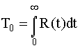
Average time to failure
T 0 = 1/ l s.(4.5.6)

Example 4.5.3. A simple system S consists of three independent elements, whose failure-free operation time distribution densities are given by the formulas:

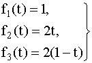at 0< t < 1 (рис. 4.5.5).

Rice. 4.5.5. Distribution densities of failure-free operation time

Find the failure rate of the system.
Solution. We determine the unreliability of each element: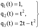
at 0< t < 1.

Hence the reliability of the elements: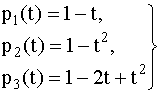
at 0< t < 1.

Failure rates of elements (conditional failure probability density) - ratio f(t) to p(t):
at 0< t < 1.
Adding, we have: l c = l 1 (t) + l 2 (t) + l 3 (t).

Example 4.5.4. Let us assume that for the operation of a system with a series connection of elements at full load, two pumps of different types are required, and the pumps have constant failure rates equal to l 1 =0.0001h -1 and l 2 =0.0002h -1 , respectively. It is required to calculate the average failure-free operation of this system and the probability of its failure-free operation for 100 hours. It is assumed that both pumps start working at time t =0.

Using formula (4.5.5), we find the probability of failure-free operation P s of a given system for 100 hours:
P s (t)= .
P s (100)=е -(0.0001+0.0002)× 100 =0.97045.

Using formula (4.5.6), we obtain

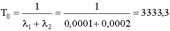h.

In Fig. 4.5.6 shows a parallel connection of elements 1, 2, 3. This means that a device consisting of these elements goes into a failure state after the failure of all elements, provided that all elements of the system are under load, and the failures of the elements are statistically independent.

Rice. 4. 5.6. Block diagram of a system with parallel connection of elements

The condition for the operability of a device can be formulated as follows: the device is operable if element 1 or element 2, or element 3, or elements 1 and 2, 1 are operational; and 3, 2; and 3, 1; and 2; and 3.

The probability of a failure-free state of a device consisting of n parallel-connected elements is determined by the theorem of addition of probabilities of joint random events as
Р=(р 1 +р 2 +...р n)-(р 1 р 2 +р 1 р 3 +...)-(р 1 р 2 р 3 +р 1 р 2 р n +... )-...± (р 1 р 2 р 3 ...р n).(4.5.7)
For the given block diagram (Fig. 4.5.6), consisting of three elements, expression (4.5.7) can be written:
R = r 1 + r 2 + r 3 - (r 1 r 2 + r 1 r 3 + r 2 r 3) + r 1 r 2 r 3 .

With regard to reliability problems, according to the rule of multiplying the probabilities of independent (collectively) events, the reliability of a device of n elements is calculated by the formula
Р = 1- ,(4.5.8)
those. when connecting independent (in terms of reliability) elements in parallel, their unreliability (1-p i =q i) is multiplied.

In the particular case when the reliabilities of all elements are the same, formula (4.5.8) takes the form
Р = 1 - (1-р) n.(4.5.9)

Example 4.5.5. The safety device, which ensures the safety of the system under pressure, consists of three valves that duplicate each other. The reliability of each of them is p=0.9. The valves are independent in terms of reliability. Find device reliability.

Solution. According to formula (4.5.9) P = 1-(1-0.9) 3 = 0.999.

The failure rate of a device consisting of n parallel-connected elements with a constant failure rate l 0 is defined as

.(4.5.10)

From (4.5.10) it is clear that the failure rate of the device for n>1 depends on t: at t=0 it is equal to zero, and as t increases, it monotonically increases to l 0.

If the failure rates of elements are constant and subject to the exponential distribution law, then expression (4.5.8) can be written

Р(t) = .(4.5.11)

We find the average failure-free operation time of the system T 0 by integrating equation (4.5.11) in the interval:

T 0 =
=(1/ l 1 +1/ l 2 +…+1/ l n )-(1/(l 1 + l 2 )+ 1/(l 1 + l 3 )+…)+(4.5.12)
+(1/(l 1 + l 2 + l 3 )+1/(l 1 + l 2 + l 4 )+…)+(-1) n+1 ´ .

In the case when the failure rates of all elements are the same, expression (4.5.12) takes the form

T 0 = .(4.5.13)

The average time to failure can also be obtained by integrating equation (4.5.7) in the interval

Example 4.5.6. Let us assume that two identical fans in an exhaust gas purification system operate in parallel, and if one of them fails, the other is capable of operating at full system load without changing its reliability characteristics.

It is required to find the failure-free operation of the system for 400 hours (the duration of the task) provided that the failure rates of the fan motors are constant and equal to l = 0.0005 h -1 , the motor failures are statistically independent and both fans start working at time t = 0.

Solution. In the case of identical elements, formula (4.5.11) takes the form
P(t) = 2exp(- l t) - exp(-2 l t).
Since l = 0.0005 h -1 and t = 400 h, then
P (400) = 2exp(-0.0005 ´ 400) - exp(-2 ´ 0.0005 ´ 400) = 0.9671.
We find the mean time between failures using (4.5.13):
T 0 = 1/l (1/1 + 1/2) = 1/l ´ 3/2 = 1.5/0.0005 = 3000 hours.

Let's consider the simplest example of a redundant system - a parallel connection of the system's backup equipment. Everything in this diagram n identical pieces of equipment operate simultaneously, and each piece of equipment has the same failure rate. This picture is observed, for example, if all equipment samples are kept at operating voltage (the so-called “hot reserve”), and for the system to function properly, at least one of the equipment must be in working order. n equipment samples.

In this redundancy option, the rule for determining the reliability of parallel-connected independent elements is applicable. In our case, when the reliability of all elements is the same, the reliability of the block is determined by the formula (4.5.9)

P = 1 - (1-p) n.
If the system consists of n samples of backup equipment with different failure rates, then
P(t) = 1-(1-p 1) (1-p 2)... (1-p n).(4.5.21)

Expression (4.5.21) is represented as a binomial distribution. It is therefore clear that when a system requires at least k serviceable ones n equipment samples, then
P(t) = p i (1-p) n-i , where .(4.5.22)

At a constant failure rate of l elements, this expression takes the form

P(t) = ,(4.5.22.1)

where p = exp(-l t).

Enabling backup system equipment by replacement

In this connection diagram n Of identical equipment samples, only one is in operation all the time (Fig. 4.5.11). When a working sample fails, it is certainly turned off, and one of the ( n-1) reserve (spare) elements. This process continues until everything ( n-1) Reserve samples will not be exhausted.

Rice. 4.5.11. Block diagram of the system for switching on backup equipment of the system by replacement
Let us accept the following assumptions for this system:
1. System failure occurs if everyone fails n elements.
2. The probability of failure of each piece of equipment does not depend on the condition of the others ( n-1) samples (failures are statistically independent).
3. Only equipment in operation can fail, and the conditional probability of failure in the interval t, t+dt is equal to l dt; spare equipment cannot fail before it is put into operation.
4. Switching devices are considered absolutely reliable.
5. All elements are identical. The spare parts have the same characteristics as new.

The system is capable of performing the functions required of it if at least one of the n equipment samples. Thus, in this case, the reliability is simply the sum of the probabilities of the system states excluding the failure state, i.e.
P(t) = exp(- l t) .(4.5.23)

As an example, consider a system consisting of two backup equipment samples switched on by replacement. In order for this system to work at time t, it is necessary that by time t either both samples or one of the two are operational. That's why
P(t) = exp(- l t) =(exp(- l t))(1+ l t).(4.5.24)

In Fig. 4.5.12 shows a graph of the function P(t) and for comparison a similar graph for a non-redundant system is shown.

Rice. 4.5. 12. Reliability functions for a redundant system with the inclusion of a reserve by replacement (1) and a non-redundant system (2)

Example 4.5.11. The system consists of two identical devices, one of which is operational, and the other is in unloaded reserve mode. The failure rates of both devices are constant. In addition, it is assumed that the backup device has the same characteristics as the new one at the beginning of operation. It is required to calculate the probability of failure-free operation of the system for 100 hours, provided that the failure rate of devices l = 0.001 h -1 .

Solution. Using formula (4.5.23) we obtain Р(t) = (exp(- l t))(1+ l t).

For given values ​​of t and l, the probability of failure-free operation of the system is

P(t) = e -0.1 (1+0.1) = 0.9953.

In many cases, it cannot be assumed that spare equipment will not fail until it is put into service. Let l 1 be the failure rate of working samples, and l 2 - backup or spare (l 2 > 0). In the case of a duplicated system, the reliability function has the form:
P(t) = exp(-(l 1 + l 2 )t) + exp(- l 1 t) - exp(-(l 1 + l 2 )t).

This result for k=2 can be extended to the case k=n. Really

P(t) = exp(- l 1 (1+ a (n-1))t) (4.5.25)
, where a = l 2 / l 1 > 0.

Reliability of a redundant system in the event of combinations of failures and external influences

In some cases, system failure occurs due to certain combinations of failures of equipment samples included in the system and (or) due to external influences on this system. Consider, for example, a weather satellite with two information transmitters, one of which is a backup or spare. System failure (loss of communication with the satellite) occurs when two transmitters fail or in cases where solar activity creates continuous interference with radio communications. If the failure rate of a working transmitter is equal to l, and j is the expected intensity of radio interference, then the system reliability function
P(t) = exp(-(l + j )t) + l t exp(-(l + j )t).(4.5.26)

This type of model is also applicable in cases where there is no reserve under the replacement scheme. For example, suppose that an oil pipeline is subject to hydraulic shocks, and the impact of minor hydraulic shocks occurs with intensity l, and significant ones - with intensity j. To break the welds (due to the accumulation of damage), the pipeline should receive n small water hammers or one significant one.

Here, the state of the destruction process is represented by the number of impacts (or damage), and one powerful hydraulic shock is equivalent to n small ones. Reliability or the probability that the pipeline will not be destroyed by microshocks at time t is equal to:

P(t) = exp(-(l + j )t) .(4.5.27)

Analysis of system reliability under multiple failures

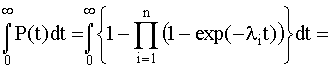
Let us consider a method for analyzing the reliability of loaded elements in the case of statistically independent and dependent (multiple) failures. It should be noted that this method can be applied to other models and probability distributions. When developing this method, it is assumed that for each element of the system there is some probability of multiple failures occurring.

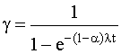
As is known, multiple failures do exist, and to take them into account, the parameter is introduced into the corresponding formulas a . This parameter can be determined based on experience in operating redundant systems or equipment and representsproportion of failures caused by a common cause. In other words, parameter a can be considered as a point estimate of the probability that the failure of some element is one of multiple failures. In this case, we can assume that the failure rate of an element has two mutually exclusive components, i.e. e. l = l 1 + l 2, where l 1 - constant rate of statistically independent element failures, l 2 - the rate of multiple failures of a redundant system or element. Becausea= l 2 / l, then l 2 = a/l, and therefore, l 1 =(1- a ) l .

We present formulas and dependencies for the probability of failure-free operation, failure rate and average time between failures in the case of systems with parallel and serial connection of elements, as well as systems with k serviceable elements from n and systems whose elements are connected via a bridge circuit.

System with parallel connection of elements(Fig. 4.5.13) - a conventional parallel circuit to which one element is connected in series. The parallel part (I) of the diagram displays independent failures in any system from n elements, and the series-connected element (II) - all multiple system failures.

Rice. 4.5.13. Modified system with parallel connection of identical elements

A hypothetical element, characterized by a certain probability of occurrence of multiple failures, is connected in series with elements that are characterized by independent failures. Failure of a hypothetical series-connected element (i.e., multiple failure) results in failure of the entire system. It is assumed that all multiple failures are completely interrelated. The probability of failure-free operation of such a system is determined as R р =(1-(1-R 1) n) R 2, where n - number of identical elements; R 1 - probability of failure-free operation of elements due to independent failures; R 2 is the probability of failure-free operation of the system due to multiple failures.

l 1 and l 2 the expression for the probability of failure-free operation takes the form

R р (t)=(1-(1-e -(1- a ) l t ) n ) e - al t ,(4.5.28)
where t is time.

The effect of multiple failures on the reliability of a system with parallel connection of elements is clearly demonstrated in Fig. 4.5.14 – 4.5.16; when increasing the parameter value a the likelihood of failure-free operation of such a system decreases.

Parameter a takes values ​​from 0 to 1. When a = 0 the modified parallel circuit behaves like a regular parallel circuit, and when a =1 it acts as one element, i.e. all system failures are multiple.

Since the failure rate and mean time between failures of any system can be determined using(4.3.7) and formulas
,
,
taking into account the expression forR p(t ) we find that the failure rate (Fig. 4.5.17) and the average time between failures of the modified system are respectively equal
,(4.5.29)
,Where .(4.5.30)

Rice. 4.5.14. Dependence of the probability of failure-free operation of a system with a parallel connection of two elements on the parameter a

Rice. 4.5.15. Dependence of the probability of failure-free operation of a system with a parallel connection of three elements on the parameter a

Rice. 4.5.16. Dependence of the probability of failure-free operation of a system with a parallel connection of four elements on the parameter a

Rice. 4.5.17. Dependence of the failure rate of a system with a parallel connection of four elements on the parameter a

Example 4.5.12. It is required to determine the probability of failure-free operation of a system consisting of two identical parallel-connected elements, if l =0.001 h -1; a =0.071; t=200 h.

The probability of failure-free operation of a system consisting of two identical parallel-connected elements, which is characterized by multiple failures, is 0.95769. The probability of failure-free operation of a system consisting of two parallel-connected elements and characterized only by independent failures is 0.96714.

System with k serviceable elements from n identical elementsincludes a hypothetical element corresponding to multiple failures and connected in series with a conventional system of the type k from n, which is characterized by independent failures. The failure represented by this hypothetical element causes the entire system to fail. Probability of failure-free operation of a modified system with k serviceable elements from n can be calculated using the formula

,(4.5.31)

where R 1 - probability of failure-free operation of an element characterized by independent failures; R 2 - probability of failure-free operation of the system with k serviceable elements from n , which is characterized by multiple failures.

At constant intensities l 1 and l 2 the resulting expression takes the form

.(4.5.32)

Dependence of the probability of failure-free operation on the parameter a for systems with two serviceable elements out of three and two and three serviceable elements out of four are shown in Fig. 4.5.18 - 4.5.20. When increasing the parameter a the probability of failure-free operation of the system decreases by a small amount(l t).

Rice. 4.5.18. The probability of failure-free operation of a system that remains operational when two of them fail n elements

Rice. 4.5.19. The probability of failure-free operation of a system that remains operational if two of the four elements fail

Rice. 4.5.20. Probability of failure-free operation of a system that remains operational when three out of four elements fail

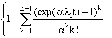
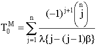
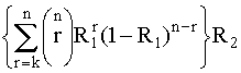
System failure rate with k serviceable elements from n and mean time between failures can be determined as follows:

,(4.5.33)

where h = (1-e -(1-b )l t ),

q = e (r a -r- a ) l t

.(4.5.34)

Example 4.5.13. It is required to determine the probability of failure-free operation of a system with two serviceable elements out of three, if l =0.0005 h - 1; a =0.3; t =200 h.

Using the expression for R kn we find that the probability of failure-free operation of a system in which multiple failures have occurred is 0.95772. Note that for a system with independent failures this probability is equal to 0.97455.

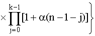
System with parallel-series connection of elementscorresponds to a system consisting of identical elements, which are characterized by independent failures, and a number of branches containing imaginary elements, which are characterized by multiple failures. The probability of failure-free operation of a modified system with a parallel-series (mixed) connection of elements can be determined using the formula R ps =(1 - (1-) n ) R 2 , where m - number of identical elements in a branch, n- number of identical branches.

At constant failure rates l 1 and l 2 this expression takes the form

R рs (t) = e - bl t . (4.5.39)

(here A=(1- a ) l ). Dependency of system failure-free operation Rb (t) for various parameters a shown in Fig. 4.5.21. At small values l t the probability of failure-free operation of a system with elements connected via a bridge circuit decreases with increasing parameter a.

Rice. 4.5.21. Dependence of the probability of failure-free operation of a system, the elements of which are connected via a bridge circuit, on the parameter a

The failure rate of the system under consideration and the mean time between failures can be determined as follows:
l + .(4.5.41)

Example 4.5.14. It is required to calculate the probability of failure-free operation for 200h for a system with identical elements connected via a bridge circuit, if l =0.0005 h - 1 and a =0.3.

Using the expression for Rb(t), we find that the probability of failure-free operation of a system with elements connected using a bridge circuit is approximately 0.96; for a system with independent failures (i.e. when a =0) this probability is 0.984.

Reliability model for a system with multiple failures

To analyze the reliability of a system consisting of two unequal elements, which are characterized by multiple failures, we consider a model in the construction of which the following assumptions were made and the following notations were adopted:

Assumptions (1) multiple failures and other failure types are statistically independent; (2) multiple failures are associated with the failure of at least two elements; (3) if one of the loaded redundant elements fails, the failed element is restored; if both elements fail, the entire system is restored; (4) the multiple failure rate and recovery rate are constant.

Designations
P 0 (t) - the probability that at time t both elements are functioning;
P 1 (t) - the probability that at time t element 1 is out of order and element 2 is functioning;
P 2 (t) - the probability that at time t element 2 is out of order, and element 1 is functioning;
P 3 (t) - the probability that at time t elements 1 and 2 are out of order;
P 4 (t) - the probability that at time t there are specialists and spare elements to restore both elements;
a- a constant coefficient characterizing the availability of specialists and spare parts;
b- constant intensity of multiple failures;
t - time.

Let's consider three possible cases of restoration of elements when they fail simultaneously:

Case 1. Spare elements, repair tools and qualified technicians are available to refurbish both elements, i.e. elements can be refurbished at the same time.

Case 2. Spare parts, repair tools and qualified personnel are only available to refurbish one item, i.e. only one item can be rebuilt.

Happening 3 . Spare parts, repair tools and qualified personnel are not available, and there may be a waiting list for repair services.

Mathematical model of the system shown in Fig. 4.5.22, is the following system of first order differential equations:

P" 0 (t) = - ,
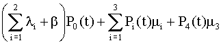P" 1 (t) = -( l 2 + m 1 )P 1 (t)+P 3 (t)

Rice. 4.5.22. Model of system readiness in case of multiple failures

Equating the time derivatives in the resulting equations to zero, for the steady state we obtain

- ,
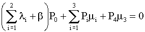-( l 2 + m 1 )P 1 +P 3 m 2 +P 0 l 1 = 0,

-(l 1 + m 2 )P 2 +P 0 l 2 +P 3 m 1 = 0,

P 2 = ,

P 3 = ,

P 4 = .

The stationary availability factor can be calculated using the formula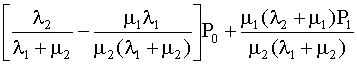

Failure rates of electrical products. It characterizes both the costs of their repairs and the amount of economic damage that occurs as a result of failures of electrical products. Objective function 3 for solving this problem is as follows  

Failure-free operation shows the property of a product to continuously remain operational for some time or some operating time, expressed in the probability of failure-free operation, average time to failure, failure rate.  

In general, the failure rate may not obey an exponential distribution law. Then the indicated expression will take the form  

Then, if the system consisted of Nu serviceable elements with a failure rate Li each, and Nd low-quality elements with a failure rate each Arf, the initial failure rate of the system (Rac) in the first period of its commissioning after repairs is equal to  

With high-quality replacement of failed elements, the failure rate of the system after the end of the running-in period increases to the value  

The failure rate is found by the formula  

An interesting analysis is presented, also based on a large amount of factual material, of two groups of gas pipeline damage that are emergency in nature, namely ruptures of gas pipeline joints and corrosion damage. The dependence of the amount of damage on the quality of work is convincingly shown, and therefore the number of failures on gas pipelines laid after 1951 is significantly lower than on gas pipelines of earlier years of laying. However, some of the article's conclusions seem overly categorical. Thus, exclusion from consideration, i.e. equating to zero, the probability of mechanical damage to gas pipelines ... since they arise from incorrect or careless work and can be prevented, as well as a complete refusal to take into account corrosion damage when determining the failure rate of gas pipelines seems to be an unjustified overestimation of the reliability of gas pipelines. The likelihood of these events has been reduced as a result of improved quality of anti-corrosion protection, improved supervision of excavation work in the gas pipeline area, etc., but still not excluded. The statement that failure can only be caused by a complete rupture of the gas pipeline joint also seems controversial. In the case of a partial rupture, the failure will be characterized by only a smaller depth. Taking into account the above, as well as the experience of Leningrad organizations, it is possible to take in calculations a value of ay that is 15-20% less than what was recommended in 1966. It is certainly desirable that the study of this issue be continued.  

I about N and A. A., Zhila V. A. Failure rate of gas pipeline sections of urban gas networks. - Gas Industry, 1972, No. 10. s, 20-25.  

Failure rate K(t) is the proportion of products that failed per unit time after a given moment, calculated in relation to the number of tested products that are operational at a given point in time.  

In practice, the failure rate is estimated using the formula  

The theoretical value of the failure rate is determined by the formula  

The failure rate indicator applies only to non-repairable products.