Formula for rectangular radio pulses. Calculation of a mathematical model of a rectangular coherent packet of rectangular radio pulses. Intrapulse modulated signals
A radio pulse is one of the most common signals in radio engineering. Therefore, studying the spectrum of a sequence of radio pulses is of particular interest.
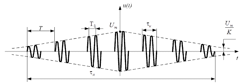
A sequence of radio pulses with a rectangular envelope, shown in Fig. 4.41 in section 4.8 can be written as:
Here are indicated:
U,w р = 2p¦ р; T r =1/¦ r; t; jn– amplitude, frequency, period, duration and initial phase of radio pulse oscillations;
W= 2pF; T = 1/F- repetition rate and repetition period of radio pulses;
n = 1, 2, 3, ...– pulse number.
In the general case, this sequence will not be strictly periodic, since the initial phases of the pulses jn can vary from pulse to pulse and the condition for the periodicity of the function is u(t)=u(t+T) - will be violated.
We will consider this general case below, but for now let us turn to the special case when the function u(t) will be purely periodic and each radio pulse will begin with the same phase j n =j=const . Let us put for definiteness j n =0 .
Coefficients of the Fourier series of this periodic function A m , B m And A 0 are found using known formulas (see Section 5.2). Index m = 1, 2, 3, ... means the harmonic number.
Since the function u(t) is symmetrical about the time axis, then A o =0. In addition, we will choose the origin of coordinates in such a way that the function u(t) (cosine) was symmetrical about the amplitude axis and was even. Then Bm =0, and, therefore, φ m =0,
Under the accepted conditions, the Fourier series of this function is:
 ,
,
will be determined only by the coefficient A m :

This is a table integral. His solution looks like:
 .
.
Substituting the limits and dividing the numerator and denominator by τ/2 , we get:
 .
.
Then the Fourier series for the function u(t) will take the form:
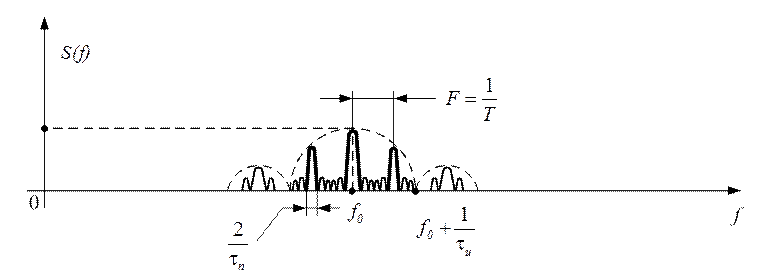
Thus, the function u(t) , which is a sequence of pulses in time, we have now presented as a sequence of frequency harmonics, which we will further call the spectrum of this function (in fact, this is not a spectrum in its classical sense, but simply another type of signal representation u(t) in time - see section 5.4).

From the resulting Fourier series it is clear that the envelope of the spectrum of a periodic sequence of radio pulses has the form sinx/x and coincides in shape with the envelope of the spectrum of rectangular video pulses (Fig. 5.6). However, the maximum of the envelope moved from zero frequency to the filling frequency of the radio pulse ω р . Spectrum harmonics are located at frequencies ± mW . Harmonic counting starts from the frequency value ω =0.
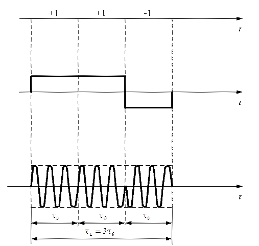
A periodic sequence of radio pulses can be obtained in two different ways.
 It is possible to “cut” radio pulses from a continuous harmonic oscillation with a period that is a multiple of the period of high-frequency filling of the radio pulses Т=kТ р
(k
- an integer), that is ω р =kW
(Fig. 5.7, a1). Let us call the resulting process a periodic sequence of radio pulses of the first type. Frequencies ω р
And W
are rigidly interconnected and therefore the maximum of the spectrum envelope coincides with the harmonic frequency kW
, which has a maximum amplitude (Fig. 5.7, a). Changing any of the frequencies ω р
or W
simultaneously changes the frequency interval between harmonics and the position of the maximum of the spectrum envelope on the frequency axis.
It is possible to “cut” radio pulses from a continuous harmonic oscillation with a period that is a multiple of the period of high-frequency filling of the radio pulses Т=kТ р
(k
- an integer), that is ω р =kW
(Fig. 5.7, a1). Let us call the resulting process a periodic sequence of radio pulses of the first type. Frequencies ω р
And W
are rigidly interconnected and therefore the maximum of the spectrum envelope coincides with the harmonic frequency kW
, which has a maximum amplitude (Fig. 5.7, a). Changing any of the frequencies ω р
or W
simultaneously changes the frequency interval between harmonics and the position of the maximum of the spectrum envelope on the frequency axis.
A periodic sequence of radio pulses can be formed at an arbitrary frequency ratio ω р And W (ω р ≠kW) . To do this, you need to select any radio pulse and “place” its copies on the time axis with a period T (Fig. 5.7, b). We will call this process a periodic radio pulse sequence of the second type.
In the spectrum of such a sequence, the position of the spectrum envelope, which has a maximum at the pulse filling frequency ω р , is not related to the position of harmonics on the frequency axis. When changing frequency ω р Only the spectrum envelope will move along the frequency axis. Harmonics will remain at frequencies mW . When changing frequency W the position of the harmonics will change, and the maximum of the spectrum envelope will remain at the frequency ω р . Thus, the position of the spectrum envelope and the position of harmonics on the frequency axis change independently. This makes it possible to select from the spectrum of a periodic sequence of radio pulses the necessary harmonic with the maximum amplitude, converting the filling frequency of the radio pulses ω р to the frequency of this harmonic (Fig. 5.7b).
The signal is a rectangular radio pulse with harmonic filling (Fig. 4.170)

When calculating the uncertainty function, we consider separately the cases of positive and negative time shifts between pulses. At

The result is similar. Summarizing the results we get
 (4.96)
Let's consider the cross section of the uncertainty function for the case f d =0. The result will be as follows
 . (4.97)
The cross section of the corresponding surface by plane f d =0 is shown in Fig. 4.171

When sectioned by the plane τ=0 we obtain
 (4.98)
The resulting formula corresponds to the modulus of the spectrum of a rectangular video pulse, which is the envelope of the original signal (Fig. 4.172).
Figure 4.163 shows the uncertainty diagram of a rectangular radio pulse

The longer the pulse duration, the higher the frequency resolution, but the worse the time resolution. The shorter the pulse duration, the higher the time resolution, but the worse the frequency resolution. This situation illustrates the principle of uncertainty in radar.
Wideband signals
A pulse signal is considered broadband if its duration is multiplied by the frequency spectrum width. There is another approach to determining the signal bandwidth. For example, in 1990 in the USA a general definition of the relative frequency band η was introduced:
![]()
In accordance with this definition, signals with a band η≤0.01 are classified as narrowband; having 0.01<η≤0,25 относится к широкополосным; имеющие 0,25<η<1 относятся к сверхширокополосным (СШП).
Pulse code sequences, linear frequency modulated signals, pseudo-noise signals, video pulses without high-frequency filling and radio pulses with high-frequency filling consisting of several periods of high-frequency oscillation can be used as UWB. The appearance of the signals is shown in Fig. 4.174.

Signal broadband is achieved by intrapulse modulation of the phase or frequency of oscillations. A wideband signal (radio pulse) has a spectrum width n times greater than a pulse of the same duration without intrapulse modulation; the width of its spectrum corresponds to a pulse without intrapulse modulation of significantly shorter duration.
Processing of broadband signals is implemented in optimal filters, the output pulses of which are determined by the amplitude-frequency spectrum of the signal. Broadband radio pulses are compressed in the optimal filter, and the greater the product, the more strongly.
Related information:
- The hidden function of witchcraft for individuals is to provide a socially accepted channel for culturally taboo expression."
Call the file AmRect. dat. Sketch the signal and its spectrum. Determine the width of the radio pulse, its height U o , carrying frequency f o, spectrum amplitude C max and the width of its lobes. Compare them with the parameters of the modulating video pulse, which you can see in Fig. 14. call from the RectVideo.dat file.
3.2.7. Radio pulse sequence
A. Call the file AmRect. dat.
B. Click
IN. Key<8>, set the signal type to "Periodic", and by clicking<Т>or
*If you activate the vertical menu button<7, F7 –T>, then the signal period can be changed using the horizontal arrows of the keyboard.
G. Go to the spectra window and press<0>(zero) move the reference point to the left. Sketch the spectrum. Record the interval value df between spectral lines and the number of lines in the spectrum lobes. Compare this data with, T and the so-called signal duty cycle Q = T/ .
E. Record the value of Cmax and compare it with that for a single signal.
Explain all results.
*3.2.8. Formation and study of am signals
The SASWin program allows you to generate signals with various and quite complex types of modulation. You are invited, using your acquired experience with the program, to generate an AM signal, the parameters and shape of which you can set yourself.
A. In the Plot option, using the mouse or cursor, create the desired type of modulation signal. It is recommended not to get carried away with its too complex form. Sketch the spectrum of your signal.
B. Save the signal to memory by pressing the vertical menu button<R AM> and assigning a name or number to the signal.
IN. Enter the Instal option and specify the signal type<Радио>. In the menu of modulation types that opens, select the Normal option of Amplitude modulation and press the button<Ок>.
G. For the query "Law of amplitude change" indicate<1.F(t) из ОЗУ>.
D. A vertical menu of signals stored in RAM will appear.
Select your signal and press the button
For example: Carrier frequency, kHz = 100,
Carrier phase = 0,
Frequency window boundaries fmin and fmax for spectrum output
Press the button
The generated signal is displayed in the left window, and its spectrum in the right.
AND. Sketch the generated signal and its spectrum. Compare them with the shape and spectrum of the modulation signal.
Z. The signal can be written to RAM or to a file and then used as needed.
AND. If desired, repeat the studies with other modulation signals.
3.3. Angle modulation
3.3.1. Harmonic modulation with small index
A. Call a signal (Fig. 15) from a file FMB0"5. dat. Sketch its spectrum. Compare the spectrum with the theoretical one (see Fig. 10, a). Note how it differs from the AM spectrum.
B. Determine the carrier frequency from the spectrum f o, modulation frequency F, initial phases O And . Measure the amplitudes of the spectrum components and use them to find the index
Rice. 15. modulation . Determine the width of the spectrum.
3 .3.2. Harmonic FM with index
>1
.3.2. Harmonic FM with index
>1
A. Call the file FMB"5. dat, where the signal with index=5 is recorded (Fig. 16). Sketch the signal and its spectrum.
B. Determine the modulation frequency F, the number of side spectrum components and its width. Find the frequency deviation f, using
Rice. 16. formula f / F. Compare the deviation with the measured spectral width.
IN. Measure the relative amplitudes С(f)/Cmax of the first three or four components of the spectrum and compare them with the theoretical values determined by the Bessel functions  . Pay attention to the phases of the spectral components.
Radio pulse carrier frequency (fill frequency):
, , ![]()
Let's determine the spectrum width Δf:
f max– determined from the graph of the amplitude spectrum of a single rectangular video pulse (Fig. 5), at a 10% level of |S(f)| max , i.e. at level 0.1|S(f)| max.
Narrowband signals (radio signals) include signals whose spectra are concentrated in a relatively narrow band compared to the average frequency. A narrowband signal is described by the expression:
ω 0 – carrier frequency
V(t), Φ(t) – signal amplitude and phase
In the special case when ![]() , and V(t)=s(t) is a non-periodic video signal, (5) describes a radio pulse:
, and V(t)=s(t) is a non-periodic video signal, (5) describes a radio pulse:
Thus, analytical expression for the received radio pulse:
Where S(t) – specified signal (see point 1)
The timing diagram of a single radio pulse is shown in Fig. 8.
The spectral density of a radio pulse is determined by the spectral density of its envelope:

The spectrum of a radio pulse U(ω) is obtained by transferring the spectrum of its envelope S(ω) from the vicinity of the zero frequency to the vicinity of the carrier frequency ±ω 0 (with a factor of 1/2):

S(2π(f–f 0)) and S(2π(f+f 0))– spectral densities of the video pulse that make up the given signal, defined in clause 1.


Amplitude spectrum of the radio pulse:
Graph for f<0 симметричен графику при в f>0 relative to the ordinate.
A graph of the amplitude spectrum of a single radio pulse is shown in Fig. 9.
4. Spectral analysis of a periodic sequence of radio pulses.
Spectral analysis of a signal in the form of a periodic sequence of radio pulses is based on its representation in the form of a Fourier series:
the coefficients of which are related to the coefficients of the Fourier series of the periodic video signal (3) by the relation:
V n – amplitude spectrum of a periodic sequence of radio pulses.
Analytical expression for a sequence of radio pulses:

U(t) – single radio pulse
The time diagram of the periodic sequence of radio pulses is presented in Fig. 10.
![]() ,
, ![]()
Let us determine the amplitude spectrum of a periodic sequence of radio pulses by:
 A graph of the amplitude spectrum of a periodic sequence of radio pulses V n is presented in Fig. 11
5.Correlation analysis of a non-periodic signal
The autocorrelation function is determined by the following integral:
 , (7)
, (7)
and characterizes the relationship between signal values at different points in time.
For a real signal, the correlation function is a real even function
![]()
The correlation function reaches its maximum value equal to the signal energy at τ=0:

Direct integration in formula (7) gives an expression for the right branch of the autocorrelation function (Fig.)
Replacement in the resulting expression τ =| τ | allows us to move on to an analytical description of the autocorrelation function, both for positive values of τ>0 and for negative τ<0.
According to the properties of the autocorrelation function
S(t±t 0), t 0 >0 => R(τ)=R(τ)
Correlation function of a burst of pulses
 , where S(t) is the 1st pulse in the burst,
provided that the repetition interval in the burst t 1 is greater than or equal to τ 0 - the duration of the 1st pulse in the burst S 0 (t) is interconnected with the correlation function R 0 (τ) by the relation
 , (8)
, (8)
Let's use expression (8):
N=2 – number of pulses
The ACF graph is shown in Fig. 12
6.Linear Circuit Spectral Analysis


Fig. 13. The given circuit diagram is Fig. 14. Equivalent equivalent circuit
CFC is determined by the following formula:

According to the equivalent equivalent circuit:
![]() ;
;
According to the voltage divider formula:
– RC circuit constant.

Let's determine the frequency response:

In contrast to the spectrum of a bell burst, the spectra of rectangular bursts have a different lobe shape, namely .
Spectra of packs of rectangular radio pulses


· The shape of the ASF arches is determined by the shape of the ASF pulses.
· The shape of the ASF petals is determined by the shape of the ASF packet.
· The spectra of bursts of video pulses are located on the frequency axis in the vicinity of low frequencies, and the spectra of bursts of radio pulses are located in the vicinity of the carrier frequency.
· The numerical value of the spectral density of pulse bursts is determined by its energy, which, in turn, is directly proportional to the amplitude of the pulses in the burst of pulse duration and the number of pulses in the burst TO(burst duration) and inversely proportional to the pulse repetition period
· With the number of pulses in a burst, the signal base (wideband coefficient) = ![]()
1.5.2. Intrapulse modulated signals
In the theory of radar it has been proven that to increase the range of a radar it is necessary to increase the duration of the probing pulses, and to improve the resolution it is necessary to expand the spectrum of these pulses.
Radio signals without intrapulse modulation (“smooth”), used as sounding signals, cannot simultaneously satisfy these requirements, because their duration and spectrum width are inversely proportional to each other.
Therefore, at present, probing radio pulses with intrapulse modulation are increasingly used in radar.
Radio pulse with linear frequency modulation
The analytical expression of such a radio signal will have the form:
where is the amplitude of the radio pulse,
Pulse duration,
Average carrier frequency,
 rate of change of frequency;
Law of frequency change.

Law of frequency change.
The graph of a radio signal with a chirp and the law of change in signal frequency within a pulse (shown in Figure 1.63 is a radio pulse with a frequency increasing over time) are shown in Figure 1.63

The amplitude-frequency spectrum of such a radio pulse has an approximately rectangular shape (Fig. 1.64)

For comparison, the ASF of a single rectangular radio pulse without intra-pulse frequency modulation is shown below. Due to the fact that the duration of a radio pulse with a chirp is long, it can be conditionally divided into a set of radio pulses without a chirp, the frequencies of which change according to the step law shown in Figure 1.65
 The spectra of each radio pulse without JIHM will each be at its own frequency:
 ![]() .
.
signal. It is easy to show that the shape of the ASF will coincide with the shape of the original signal.
Phase-code-manipulated pulses (PCM)
FCM radio pulses are characterized by an abrupt change in phase within the pulse according to a certain law, for example (Fig. 1.66):
three-element signal code
phase change law
three-element signal
or seven-element signal (Fig. 1.67)
Thus, we can draw conclusions:
· ASF of signals with chirp is continuous.
· The ASF envelope is determined by the shape of the signal envelope.
· The maximum ASF value is determined by the signal energy, which in turn is directly proportional to the amplitude and duration of the signal.
The spectrum width is ![]() where the frequency deviation and does not depend on the signal duration.
where the frequency deviation and does not depend on the signal duration.
Signal base (wideband ratio) ![]() May be n>>1. Therefore, chirp signals are called broadband.
May be n>>1. Therefore, chirp signals are called broadband.
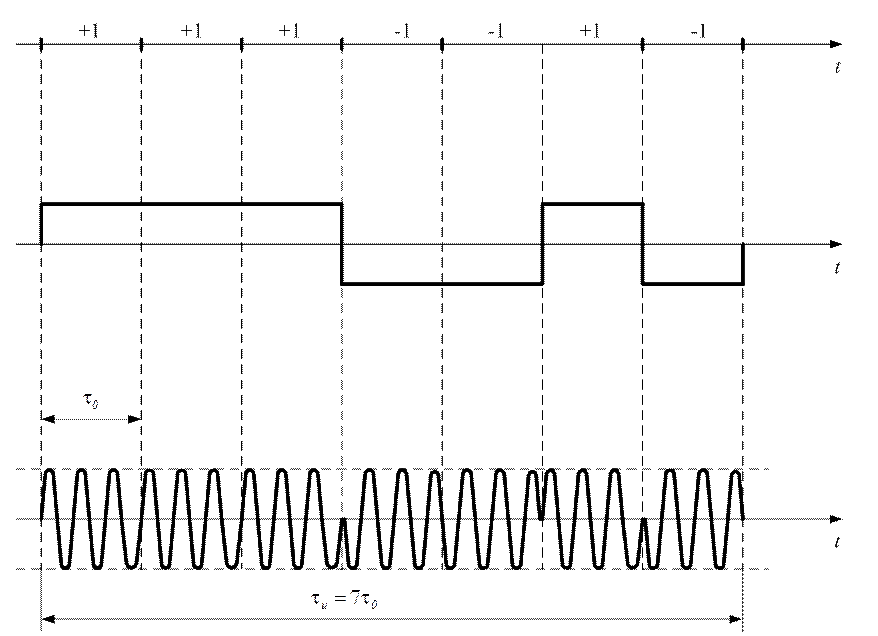
FCM radio pulses with a duration are a set of elementary radio pulses following each other without intervals, the duration of each of them is the same and equal to  . The amplitudes and frequencies of the elementary pulses are the same, but the initial phases may differ by (or some other value). The law (code) of alternation of initial phases is determined by the purpose of the signal. For FCM radio pulses used in radar, appropriate codes have been developed, for example:
1, +1, -1 - three-element codes
 - two variants of four-element code
1 +1 +1, -1, -1, +1, -2 - seven-element code
The spectral density of coded pulses is determined using the additivity property of Fourier transforms, in the form of the sum of the spectral densities of elementary radio pulses.
ASF graphs for three-element and seven-element pulses are shown in Figure 1.68

As can be seen from the figures above, the width of the spectrum of PCM radio signals is determined by the duration of the elementary radio pulse
 or .
or .
Broadband coefficient  , Where N-the number of elementary radio pulses.
2. Process analysis using time methods. General information about transient processes in electrical circuits and the classical method of their analysis
2.1. The concept of transition mode. Commutation laws and initial conditions
Processes in electrical circuits can be stationary and non-stationary (transient). A transient process in an electrical circuit is a process in which currents and voltages are not constant or periodic functions of time. Transient processes can occur in circuits containing reactive elements when connecting or disconnecting energy sources, abrupt changes in the circuit or parameters of incoming elements (switching), as well as when signals pass through the circuits.  In the diagrams, switching is indicated in the form of a key (Fig. 2.1); it is assumed that switching occurs instantly. The moment of commutation is conventionally taken as the beginning of the time count. In circuits that do not contain energy-intensive elements L and C during switching, transient
there are no processes. In circuits with energy-intensive elements, transient processes continue for some time, because energy stored by the capacitor  or inductance
  cannot change abruptly, because this would require an energy source of infinite power. In this regard, the voltage across the capacitor and the current through the inductance cannot change abruptly. Designating