Digital image interpolation. Educational program: image resizing methods

To increase or decrease the size of an image, Photoshop uses the Interpolation method. So, for example, when you enlarge an image, Photoshop creates additional pixels based on the values ​​of neighboring ones. Roughly speaking, if one pixel is black and another is white, then Photoshop will calculate the average and create a new gray pixel. Some types of interpolation are fast and poor quality, others are more complex, but they achieve good results.

First, let's go to the main menu Image - Image Size or Alt+Ctrl+I.

If you click on the arrow next to the parameter Resample Image, then several interpolation options will appear in the pop-up window:

• Automatic. Photoshop application selects a resampling method based on the document type and upscaling or downscaling.
• Preserve details (enlargement). When this method is selected, the Noise Reduction slider becomes available to smooth out noise when the image is scaled.
• Preserve Details 2.0. This algorithm gives very interesting result enlarge the picture. Of course, the detail does not become more detailed, but what is there increases quite significantly without losing clarity.
• . Good method for image enlargement based on bicubic interpolation, designed specifically for smoother results.
• Bicubic Sharper (reduction). A good method for reducing image size based on bicubic interpolation with increased sharpness. This method allows you to preserve details of the resampled image. If Bicubic Down interpolation makes some areas of the image too sharp, try using Bicubic interpolation.
• Bicubic (smooth gradients). Slower, but also more exact method, based on analysis of the color values ​​of surrounding pixels. By using more complex calculations, bicubic interpolation produces smoother color transitions than neighbor interpolation or bilinear interpolation.
• Nearest Neighbor (hard edges). A quick but less accurate method that follows the pixels of an image. This method preserves sharp edges and produces a reduced file size in artwork that contains unsmoothed edges. However, this method can create jagged edges that become noticeable when you distort or scale the image, or perform many selection operations.
• Bilinear. This method adds new pixels by calculating the average color value of surrounding pixels. It produces results of average quality.

Usage example Bicubic Smoother (enlargement):

There is a photo, dimensions 600 x 450 pixels, resolution 72 dpi

We need to increase it. Opens a window Image Size and choose Bicubic Smoother (enlargement), units of measurement are percentages.

The document dimensions will immediately be set to 100%. Next, we will gradually enlarge the image. Change the value from 100% to 110%. When you change the width, the height will automatically adjust itself.

Now its dimensions are already 660 x 495 pixels. By repeating these steps you can achieve good results. Of course, it will be quite difficult for us to achieve ideal clarity, since the photo was small and low resolution. But look at the changes that have taken place in the pixels.

How big can we make photos with interpolation? It all depends on the quality of the photo, how it was taken and for what purpose you are enlarging it. Best answer: take it and check it yourself.

See you in the next lesson!

Image interpolation occurs in all digital photographs at a certain stage, be it dematrization or scaling. It occurs whenever you change the size or scan of an image from one grid of pixels to another. Resizing an image is necessary when you need to increase or decrease the number of pixels, while changing the position can occur in the most various cases: Correct lens distortion, change perspective, or rotate the image.

Even if the same image is resized or scanned, the results can vary significantly depending on the interpolation algorithm. Since any interpolation is just an approximation, the image will lose some quality whenever it is interpolated. This chapter aims to provide a better understanding of what affects the results - and thereby help you minimize any loss of image quality caused by interpolation.

Concept

The essence of interpolation is to use available data to obtain expected values ​​at unknown points. For example, if you wanted to know what the temperature was at noon, but measured it at 11 o'clock and at one o'clock, you can guess its value by applying linear interpolation:

If you had an extra measurement at half past twelve, you could notice that the temperature rose faster before noon and use that extra measurement to perform a quadratic interpolation:

The more temperature measurements you have around midday, the more complex (and expectedly more accurate) your interpolation algorithm can be.

Example of resizing an image

Image interpolation works in two dimensions and tries to achieve the best approximation in pixel color and brightness based on the values ​​of surrounding pixels. The following example illustrates how scaling works:

original before after without interpolation

Unlike fluctuations in air temperature and the ideal gradient above, pixel values ​​can change much more dramatically from point to point. As with the temperature example, the more you know about the surrounding pixels, the better the interpolation will work. This is why the results quickly deteriorate as the image is stretched, and also why interpolation can never add detail to an image that is not there.

Image rotation example

Interpolation also occurs every time you rotate or change the perspective of an image. The previous example was misleading because it special case, in which interpolators usually work well. The following example shows how quickly detail can be lost in an image:

original turn by 45 turn by 90 (without loss) 2 turns by 45° 6 turns by 15°

A 90° rotation introduces no loss, since no pixel needs to be placed on the border between two (and therefore divided). Notice how much of the detail is lost on the first turn, and how the quality continues to drop on subsequent turns. This means that rotations should be avoided as much as possible; If an unevenly exposed frame requires rotation, you should not rotate it more than once.

The above results use the so-called "bicubic" algorithm and show a significant degradation in quality. Notice how the overall contrast decreases due to the decrease in color intensity, how dark halos appear around the light blue. The results can be significantly better depending on the interpolation algorithm and the imaged subject.

Types of interpolation algorithms

Common interpolation algorithms can be divided into two categories: adaptive and non-adaptive. Adaptive methods vary depending on the subject of interpolation (hard edges, smooth texture), while non-adaptive methods treat all pixels equally.

Non-adaptive algorithms include: nearest neighbor, bilinear, bicubic, splines, sinc, Lanczos and others. Depending on complexity, they use from 0 to 256 (or more) contiguous pixels for interpolation. The more adjacent pixels they include, the more accurate they can be, but this comes at the cost of a significant increase in processing time. These algorithms can be used for both scanning and scaling of images.

Adaptive algorithms include many commercial algorithms in licensed programs such as Qimage, PhotoZoom Pro, Genuine Fractals, and others. Many of them use different versions of their algorithms (based on pixel-by-pixel analysis) when they detect the presence of a border - with the goal of minimizing unsightly interpolation defects in the places where they are most visible. These algorithms are primarily designed to maximize the defect-free detail of enlarged images, so some of them are not suitable for rotating or changing the perspective of an image.

Nearest neighbor method

This is the most basic of all interpolation algorithms and requires the least processing time because it only takes into account one pixel - the one closest to the interpolation point. As a result, each pixel simply becomes larger.

Bilinear interpolation

Bilinear interpolation considers a 2x2 square of known pixels surrounding an unknown one. The weighted average of these four pixels is used as the interpolated value. The result is images that look significantly smoother than the result of the nearest neighbor method.

The diagram on the left is for the case where all known pixels are equal, so the interpolated value is simply their sum divided by 4.

Bicubic interpolation

Bicubic interpolation goes one step further than bilinear interpolation, looking at a 4x4 array of surrounding pixels - 16 in total. Since they are on different distances from an unknown pixel, the nearest pixels receive more weight in the calculation. Bicubic interpolation produces significantly sharper images than the previous two methods and is arguably the best in terms of processing time and output quality. For this reason, it has become standard in many image editing programs (including Adobe Photoshop), printer drivers and built-in camera interpolation.

Higher order interpolation: splines and sinc

There are many other interpolators that take more surrounding pixels into account and thus are more computationally intensive. These algorithms include splines and cardinal sine (sinc), and they retain most of the image information after interpolation. As a result, they are extremely useful when an image requires multiple rotations or perspective changes in separate steps. However, for single increments or rotations, such higher-order algorithms provide negligible visual improvement with a significant increase in processing time. Moreover, in some cases, the cardinal sine algorithm performs worse on a smooth section than bicubic interpolation.

Observable interpolation defects

All non-adaptive interpolators try to find the optimal balance between three undesirable defects: boundary halos, blur, and aliasing.

original aliasing blur halo

Even the most developed non-adaptive interpolators are always forced to increase or decrease one of the above defects at the expense of the other two - as a result, at least one of them will be noticeable. Notice how the edge halo looks like an artifact caused by sharpening with an unsharp mask, and how it increases the apparent sharpness by sharpening.

Adaptive interpolators may or may not create the defects described above, but they can also produce textures or single pixels at large scales that are unusual for the original image:

Material with small texture Area at 220% magnification

On the other hand, some “defects” of adaptive interpolators can also be considered as advantages. Because the eye expects to see detail down to the smallest detail in finely textured areas such as foliage, such patterns can deceive the eye at a distance (for certain types of material).

Smoothing

Anti-aliasing or anti-aliasing is a process that attempts to minimize the appearance of jagged or jagged diagonal borders that give text or images a rough digital appearance:

Anti-aliasing removes these steps and creates the appearance of softer edges and high resolution. It takes into account how much the ideal border overlaps adjacent pixels. A jagged border is simply rounded up or down with no value in between, while a smooth border produces a value proportional to how much of the border is included in each pixel:

An important consideration when enlarging images is to avoid excessive aliasing resulting from interpolation. Many adaptive interpolators detect the presence of edges and adjust to minimize aliasing while maintaining edge sharpness. Since a smoothed boundary contains information about its position at a higher resolution, it is possible that a powerful adaptive (edge-detecting) interpolator can at least partially reconstruct the boundary when zoomed in.

Optical and digital zoom

Many compact digital cameras can perform both optical and digital magnification (zoom). Optical zoom is achieved by moving the vari-lens so that the light is amplified before it hits the digital sensor. In contrast, digital zoom reduces quality because it simply interpolates the image after it has been received by the sensor.

Optical zoom (x10) Digital zoom (x10)

Even though a photo using digital zoom contains the same number of pixels, its detail is distinctly less than when using optical zoom. Digital zoom should be eliminated almost entirely, except in cases where it helps display a distant subject on your LCD screen. cameras. On the other hand, if you typically shoot in JPEG and want to crop and enlarge your image later, digital zoom has the advantage of interpolating before introducing compression artifacts. If you find that you need the digital zoom too often, invest in a teleconverter or, better yet, a longer focal length lens.

An image digitized on a scanner is presented on a computer monitor during the editing process and processed in an editor to produce a high-quality printed version. This chain of operations is so familiar to most users that few people think about the difficult transformations that the original undergoes along this path.

The screen version of the image is simply a matrix of dots, which is described by its dimensions in height and width. An image with dimensions of 600 by 400 will occupy a fixed proportion of screen space on any monitor, regardless of its operating principle. It will cover almost the entire screen if the resolution is 640*480, on a screen with a resolution of 1024*768 it will take up about a quarter of the space, and finally, with a resolution of 1600*1200 it will take up a little more than one-ninth of the screen area. At the same time, the physical dimensions, i.e. dimensions, which are calculated in inches and centimeters, will depend on the diagonal of the monitor.

What will be the size of the image when it is printed? For an experienced Photoshop user, the answer is obvious. The dimensions of the printed version coincide with the dimensions of the scanned original (to be extremely precise, with the dimensions of the scanning area). This natural convention is the default setting for all graphics programs; but most raster editors have by special means changing print sizes.

To set the size of the screen version of the image, which coincides with its printed version, you need to execute the main menu command View - Print Size Photoshop editor or use the panel button with the same name.

Let's say you want to print an image with a size of 600*600 pixels. These dimensions are a given, now the method of obtaining them, scanning resolution and printing installation does not matter. If you set the dimensions of the printed version to 10 inches, the resolution will be 600 dot / 10 inch = 60 dpi. Here are a number of resolution values ​​for different print sizes:

• 600dot/5inch = 120dpi;
• 600dot / 3inch = 200dpi;
• 600dot / 2inch = 300dpi.

All these changes do not affect the screen version at all; all its advantages and disadvantages are introduced at the scanning stage and changes in the printing area do not affect the quality of the digitized original. But this has a significant impact on the quality of the printed version.

For any printing equipment there is some optimal resolution value digital image, when the printing device will be able to convey the maximum number of details of the original. The quality of the result also depends on the type of paper chosen. This influence is especially strong for the most popular in our time printing devices- color inkjet printers.

Let the optimal resolution value for the selected printer and type of paper be 200 dpi. What consequences will result from printing the selected original with a resolution of 120 dpi? This solution will lead to a loss of quality, since some of the details will be lost during printing. What if you compete for results by choosing a higher print resolution? If, for example, you set it to 300 dpi or more, then redundant information will be transmitted to the printer, which it simply cannot use.

Let's say that the scanned version of the image shows mediocre quality when displayed on the monitor. Is it possible to improve the situation by printing it on high-quality paper with high resolution? The trick will not work because printing does not add new information to the original; the printer uses only the data that was included in the image at the digitization stage. These thought experiments, of course, simplify real situation affairs, but the action of the principle of reasonable sufficiency for choosing the optimal print resolution can hardly be disputed.

So, if you fix the point dimensions of the image, then any changes in resolution entail a modification of the print area. The opposite statement is also true. IN raster graphics this transformation is usually called scaling.

Why scale the image? The reasons for this are varied and often very compelling. Many of today's mid-range digital cameras produce small images that, when printed, take up the space of a postage stamp. Desktop Publishing require images of fixed dimensions, which may not coincide with the original dimensions, etc.

Scaling does not change physical dimensions graphic file, since it does not affect any of the parameters (number of dots, color depth) on which its value depends.

Sampling

Changing the number of image points is called sampling. This operation obviously affects the size of the screen version of the image, which on a monitor with unchanged characteristics becomes larger or smaller, depending on the specified values.

Rice. 2.4.

Let us explain this operation using an example of an image from the editor’s standard collection (Fig. 2.4). The original version of the picture, which occupies the middle position, has a resolution of 72 dpi. Doubling the resolution to 144 dpi entails an increase in the number of pixels and an increase in the linear dimensions of the screen version of the image (right sample). Reducing the resolution to 36 dpi produces exactly the opposite effects (left sample).

Unlike upscaling, sampling is not a computationally straightforward operation because it strongly interferes with the structure of the image.

Let there be an image of size 400*400 pixels. If you reduce its screen size to 300*300, then, at first glance, this means a slight intervention in the original - a reduction of only three quarters. A different picture emerges if you count the number of points before and after surgery. The original image consisted of 400*400 = 160,000 pixels, and after transformation it has 300*300 = 90,000 pixels - almost half as much. It is clear that such a large-scale operation cannot but affect the quality of the picture.

Even more complex problems have to be solved when the number of points increases. If, when reducing them, the program simply discards extra pixels, then when increasing the matrix, additional points must be “invented”. Adding new pixels is performed using special interpolation algorithms.

Reducing the number of image pixels is a relatively safe procedure that does not directly affect the quality of the original. Increasing the pixels is more complex in its algorithms and consequences. A small increment in the raster does not entail noticeable negative consequences. This kind of large-scale conversion almost always degrades the sharpness of the image, partially blurring the image.

In raster graphics, three main sampling methods have become widespread (all of them are supported by the Photoshop editor), which differ in speed and accuracy of results:

• Nearest Neighbor(By adjacent pixels). The simplest interpolation method with high speed work and results are not of the highest quality. The characteristics of its nearest actual neighbor are taken as a sample for a new pixel. The method gives good results for areas with regular geometry, such as straight lines, rectangles, etc.;
• Bilinear(Bilinear). This method is somewhat more difficult to implement, but gives best results compared to the method Nearest Neighbor. Options new point are calculated by averaging the color or tone characteristics of adjacent real image pixels. The method shows its advantages when the number of image pixels is reduced. A rational area of ​​its application is the processing of images of average quality;
• Bicubic(Bicubic). This best method interpolation, which is why it is the default in Photoshop. New points are calculated from existing neighbors using slightly more complex algorithms than in the previous method;
• Bicubic Smoother(Bicubic with smoothing). A variant of the bicubic interpolation method. It is designed to sample high quality images while increasing their size;
• Bicubic Sharper(Bicubic with sharpness adjustment). A variant of the bicubic interpolation method. It is designed to process high-quality images while reducing their size.

What happens to the resolution and print area when the sampling procedure is performed? The answer gives the definition of resolution: Length ( inch ) * Resolution (dpi)= Number of dots.

This relationship shows that any image sampling must change its actual length or resolution. From a mathematical point of view, both possibilities are equal; it is only important to maintain the equality of the right and left sides of the equation. When you resample an image in Photoshop, the print dimensions change, but the resolution remains the same. By slightly more complex manipulation of the number fields in the same dialog box, you can compensate for the change in the number of points using new resolution values.

The sampling operation can also be performed by digitizing devices. When processing an original at a resolution that is not an integer part of the maximum optical scanner resolution A procedure has been implemented that is in many ways reminiscent of bilinear interpolation performed by raster editors when changing the number of image pixels. Let's look at this situation in more detail. Suppose you want to digitize an original three inches wide on a scanner with a maximum optical resolution of 600 dpi. By simple multiplication you can find the number of photosensitive ones that will be involved in this procedure. It is equal to 600 * 3 = 1800. If the resolution is set to half the maximum (300 dpi), then 900 sensors will participate in the digitization process, i.e. every other. Operation in this mode can be organized using elementary means, without making deep changes to the device control algorithms. A completely different situation arises if you choose a digitization density that is not an integral part of the maximum optical resolution. This will lead to a violation of the regularity of the location of active sensors, so the true appearance of the scanned original can only be formed with the participation of special corrective algorithms working on the principle of software interpolation.

The choice of scanning resolution is often justified by rational arguments, but despite strong physical arguments and logical reasoning, the user almost always remains with significant freedom of choice. Even in a thought experiment, it is difficult to imagine a situation where it is impossible to deviate from the calculated scanning resolution. In most cases, image quality does not undergo critical changes even with significant resolution deviations from the calculated optimal values. Therefore, you should choose a digitization density that approximates the calculated value from above and at the same time is an integral part of the maximum optical resolution of the selected scanning device. In other words, if the scanner is capable of operating at a resolution of 300 dpi, then multiples of 75, 100, 150 dpi are preferable to scan settings that are not an integer part of 300, such as 120 or 175 dpi. If for some original, using calculation or other means, it is obtained optimal resolution, equal to 140 dpi, then in a real scanning session it is advisable to set 150 dpi.

Let us note once again the fundamental differences between scaling and sampling. The first operation only affects the printed version of the image, it does not affect the actual pixels in any way, so screen version the image does not undergo any changes even with significant scale transformations. Its results can only be seen when the document is printed. The second operation is more complex in technique and more responsible in its results. It performs a deep restructuring of the image, under certain conditions, affecting each of its pixels.

In the English-language literature, a subtle terminological distinction is often made between increasing and decreasing the number of points. The first operation is called upsampling, and the second is called downsampling, and the generic term is resampling. In Russian literature you can find a literal, tracing translation of these operations into Russian - upsampling, downsampling and resampling! If you can still come to terms with the last term, then the first two words clearly do not agree with the structure of Russian speech and their existence is not dictated by technical necessity.

Scaling and sampling in Photoshop

Photoshop is a professional raster editor, so it fully supports scaling and sampling functions. All possible operations of this type are performed using one Image Size dialog box. To display it on the screen, just run the command Image - Image Size (Fig. 2.5).

Let's look at the main features of this window:

• Pixel Dimensions. This section displays the image dimensions, specified in pixels or percentages, and the total size of the current document in kilobytes or megabytes. The fields in this section are available when the Resample Image option is active. Otherwise, the program prohibits direct changes to these values;
• Document Size. This section displays information about the actual dimensions of the printed print and the resolution at which the image receives its current dimensions. These fields can be directly modified. An increase in the size of the printed print entails an increase in the number of pixels in the digital version of the image and vice versa;
• Constrain Proportion(Keep proportions). This option controls the preservation of document proportions. If it is enabled, then any operations with the image will preserve the original aspect ratio. If the option is not selected, then the dimensions of the sides can be changed independently of each other.
• Resample Image (Interpolation). This option controls the sampling process. If it is enabled, the program allows you to change the point size of the original, and therefore the total number of pixels, at the user's discretion. Otherwise, all fields in the Pixel Dimension section become unavailable, and dimensions are controlled only by adjusting the printed size or resolution.
• Raster resizing is performed using interpolation algorithms. To select the interpolation method, use the nameless list located next to the switch. You can choose one of five available methods Nearest image recalculation Neighbor(By adjacent pixels), Bilinear (Bilinear) and three variants of the Bicubuc method (Bicubic). The features of these sampling algorithms were discussed in the previous section.

If manipulations with the settings of the Image Size dialog box were unsuccessful, you can reset them and return to the starting parameter values. To do this, press and hold Alt key, as a result, the Cancel button will turn into Reset, which serves to discard the changes made to the window. This standard editor technique is used in many program dialogs.

What reasons force you to resort to scaling? It is impossible to mention all the situations in which this technique is necessary. Let's give just one example. Many digital cameras produce low-resolution and large-sized originals. Let the image be obtained with a resolution of 72 dpi and dimensions of 30 by 20 centimeters. If you send it for printing in this condition, the quality of the print will be low. We can confidently predict the appearance of irregularities at the edges of lines and clearly visible steps in areas with smooth color transitions. The number of dots in the original is large enough (almost half a million) to produce a high-quality printed version. You just need to reduce the size of the printed version. To do this, you need to disable the Resample Image option and enter reasonable print sizes in the Document Size section fields, for example, 10 centimeters in width. The program will recalculate all other available parameters. The height will be 6.5 cm, and the resolution will be 215. These values ​​guarantee printing of sufficiently high quality.

Key terms

Bicubic interpolation- interpolation method in which new points bitmap are created from the color and brightness values ​​of several neighboring pixels. This interpolation method is based on a more complex calculation algorithm than the nearest neighbor method, so it requires more computational resources but produces better results.

Color depth- the total number of binary bits per pixel of a raster image. Let some image be recorded in the RGB system, and 8 binary bits (1 byte) are allocated for each chromatic coordinate R, G, and B. One could argue that this image has a color depth of 8 bits per channel or 3 * 8 = 24 bits per pixel.

Sampling- changing the number of pixels of the raster image.

Interpolated Resolution- characteristics of digitizing devices in which digital image points are obtained by a combination of physical reading and software interpolation.

Bitmap Interpolation- procedure for calculating and adding new points to a raster image.

Scaling a bitmap- changing the resolution of the image when displaying it on various media, provided that the point dimensions of the original are preserved.

Nearest neighbor method- an interpolation method that generates new points in a raster image, borrowing color and brightness characteristics from the nearest neighboring point. The fastest and crudest interpolation method.

Mechanical resolution- characteristic of flatbed scanners equal to the vertical sampling density. This parameter is usually equal to the minimum carriage offset of the flatbed scanner, and is therefore called vertical resolution.

Optical resolution- characteristic of flatbed scanners equal to the density of photoreceptors. This parameter is sometimes called horizontal resolution.

Digitization- procedure for converting an image into raster electronic form.

Image Resolution- characteristic of a raster image that specifies the density of dots (pixels) per unit length. Usually measured in dots per inch inch, dpi) or pixels per inch inch, ppi).

Permission digital camera - the total number of receptors of the photosensitive matrix, for example 8 megapixels = 8 million pixels.

Screen resolution- two numbers equal to the maximum number of independent addressable points in width and height, for example 800*600, 1024*768.

True Color color space- RGB color space with a color depth of 24 bits per pixel. The set of colors in this space is 16,777,216. This palette is sufficient to represent and process most digital images in electronic publishing and printing.

To understand what processes are involved in the mechanism for resizing an image, read the building material of any raster image. In short, these are small colored squares that, like a mosaic, make up a picture.

When we talk about sizes, we say about permission. It is written as the sum of pixels in one row in width and one column in height and is written like this: 655x382. These are the dimensions of the following art:

Therefore, when resizing the image, we must change the values ​​of these pixels in width and/or height.

In case of size reduction, for example, let's change our example to 300x175, the image will already consist of 300 pixels in width and 175 pixels in height. No narrowing occurred. Photoshop recalculated the pixels in the image and figured out which ones it could get rid of.

But this process is not reversible. If you need to return everything back or do even more, then a new process will start - increase.

In case of increasing size, Photoshop calculates which pixels are missing and adds them based on complex processing algorithms. This process cannot be of high quality, so when the image is enlarged, the quality is lost. The picture loses the clarity of details and becomes blurry. For clarity, I will increase the example above to original size. Compare:

Thus, when enlarging, the quality will greatly depend on the initial size of the image and on the course to which you need to “grow”.

Image Size Dialog Box

So, the most basic way to resize an image is to use the menu command:

Image - Image Size.

Hotkey: Alt+Ctrl+I.

A dialog box will open:

This dialog box allows you, firstly, to obtain information about the current image dimensions, and secondly, to actually change them.

Pixel Dimensions

To change the image size change the values Width and Height. By default they are measured in pixels, but you can select percentages from the drop-down list.

Notice the bracket and chain icon. This means that when you change the width or height, the second value will automatically change in the same proportions as the original image. This is necessary so that it does not turn out compressed or elongated. To enable/disable this function, check the box. "Keep proportions"(Constrain Proportions).

Document Size

I mentioned this group of settings when talking about the printer. Permission(Resolution) changes the pixel size and affects print quality. For printers, feel free to set it in the range of 200-300 pixels per inch.

The Width and Height values ​​tell us what sizes of paper the image can be printed on. Changing the numbers will change the size of the image. Please note that there is also a function for maintaining proportions.

Scale Styles

Determines whether the program will scale any layer styles applied to the image. It is recommended to leave this option checked, otherwise, for example, the shadow you added may end up being larger or smaller than the picture itself.

Interpolation

This is your key to changing resolution without affecting image quality. Interpolation Resample Image is the process by which Photoshop responds to a resizing command by adding or subtracting pixels. The problem is that when interpolating, the program “makes assumptions”, and this can ruin the quality of the image.

When you first start the program, setup Interpolation is turned on, and is responsible for increasing or decreasing the number of pixels in the image. These processes reduce image quality as the program either creates pixels or chooses which ones to remove accordingly. By disabling the setting, you protect quality by locking the pixel size.

When you check the box Interpolation, you need to select a method from the drop-down list below. Why might this be needed? Sometimes you'll need Photoshop's help to create an image larger or smaller than the original.

For example, if you have an image with the resolution 200 pixels per inch, the size of which when printed is 4x6, and the size of the printed version should be 5x7 and it is advisable to keep the resolution at 200 pixels per inch. To do this, you can check this box.

The drop-down options below the Interpolation check box determine what form of math Photoshop uses to add or remove pixels. Since more high quality images means more work, how better picture, the more time the program needs to complete the above process.

Here are your options, sorted by quality (worst to best) and speed (fastest to slowest):

• By neighboring pixels (preserves sharp edges) (Nearest Neighbor). Although this method results in the most low quality images, it can be useful because it creates the smallest files. This is useful if you are transferring files over the Internet and you or the recipient has a slow connection. This method works by looking at the colors of surrounding pixels and copying them. It is known for creating jagged edges, so you should only apply it to images with hard edges, such as illustrations, that have not been smoothed.
• Bilinear. If you choose this method, Photoshop will guess the color of the new pixels, choosing a middle ground between the color of the pixels directly above and below, and to the left and right of the one being added. The result of this method is slightly better than when choosing the option By neighboring pixels and it's still pretty fast, but you're better off using one of the following three methods instead of Bilinear.
• Bicubic (best for smooth gradients). This method determines the colors of new pixels by averaging the colors of the pixels directly above and below the new one, as well as the two pixels to the left and right of it. This method takes longer than the previous two, but creates a smoother transition in areas where one color is replaced by another.
• Bicubic Smoother (best for enlargement). Close to the previous method in the way new pixels are created. Using this method, the pixels are slightly blurred so that new ones can be superimposed on old ones, giving the image a smoother, more natural look. Recommended use this method to enlarge images.
• Bicubic Sharper (best for reduction). This method is also similar to the method Bicubic (best for smooth gradients) in the way it creates new pixels, but instead of blurring entire pixels to improve the blending of new and old like the previous method, it only softens the edges of the pixels. It is recommended to use this method to reduce images.

Wait! We forgot something! So far we've been talking about "real" or optical resolution (even though it may not be as real as you thought). Resolution can also be faked using various mathematical algorithms, giving an apparent resolution that is higher than the figure given for optical resolution. This process is called interpolation.

In the bad old days, many vendors would have preferred to quote the interpolated resolution value as a specification if they had known it. At that time, resolution was lower (before the advent of affordable film scanners), so the temptation was very great. So for flatbed scanners, which are used to obtain images of photographs and similar products, the actual optical resolution could be 300x300 samples per inch. Using the magic of interpolation, the same scanner could produce a fake resolution of 600x600 samples per inch or even 1200x1200 samples per inch. And that's what the sellers would advertise. Gullible buyers might think they are buying a scanner with 1200x1200 samples per inch resolution, when much of the extra clarity would be mathematical "witchcraft".

Fortunately, almost no one engages in such fraud. All vendors list the optical resolution of their scanners as the primary specification for clarity, even though, as you have seen, the optical resolution may not accurately reflect the resolution of the scanner. The interpolated resolution is hidden in other specifications in a way that makes them seem much less deceptive.

Even so, many scanner users do not fully understand what interpolation is and either trust it too much or, conversely, too little. In fact, although interpolated resolution is not as good as optical resolution, when correct use it may be quite useful.

Interpolation is nothing more than a process that is used during scanning to change the image size (up or down) or color saturation to some other value different from the size or color saturation of the original. While interpolation can be used to change color information or make a scanned image smaller than the original, most talk about interpolation refers to the image in which new pixels are created, causing the final image to be larger or have a higher resolution than the scanned original. (Interpolation, which is used to make an image smaller, is commonly called downsampling.)

Don't confuse interpolation with rescaling. When you zoom in on an image, each pixel is duplicated a certain number of times. To triple the image size, each pixel is duplicated three times. The same thing happens when you zoom out. With simple rescaling, reducing the image size by one-third of the original means discarding every third pixel (in the hope that the remaining pixels will still retain some semblance of the original). Either way, the resulting image will likely have rough edges or "ladders" on the diagonal lines.

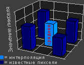
Interpolation is a much more complex process. Instead of simply copying pixels, interpolation algorithms are used to study neighboring pixels and calculate new ones, which are adjusted so that the transition between them is as imperceptible as possible, ideally forming a continuous transition from old pixels to new ones. Simplified, this process can be described as follows. If there was a black pixel in the image and a white one next to it, then if you zoomed in twice, you would get two black pixels and two white pixels. When interpolated, we get the original black and white pixels, plus one dark gray pixel and one light gray pixel in between, as shown in Fig. 3.3.

There are various ways image interpolation, some of them quite complex. Below are the three most common methods.

- Nearest neighbors method. With this method, a pixel located in close proximity to the one being processed is considered, and information about this pixel is used to create a new one.

Since in this case you only need to check every second pixel, this is a fairly fast method, although not very accurate. It is not suitable for most photographic images containing smooth transitions between individual areas, since it gives them noticeably more jagged edges. If you are scanning an image with clear edges, such as a piece of text or an image that will be saved in GIF format, the nearest neighbors algorithm will be quite suitable. In such cases, it produces smaller files while effectively maintaining sharp edges. In Fig. 3.4 shows the letter A (one of the types of images for which the nearest neighbors algorithm works quite well), and in Fig. Figure 3.5 shows a part of this letter enlarged by 600% after processing using this.

- Bilinear method. This method checks the pixels on either side of the pixel being processed. It is slightly slower than the nearest neighbor algorithm, but can produce reasonably good results for images containing high-contrast elements. The operation of the corresponding algorithm is shown in Fig. 3.6.

- Bicubic method. The most common interpolation method is bicubic, in which all surrounding pixels are examined to obtain information for creating new, interpolated pixels. This is the default method in many scanners, as well as Photoshop. The latest version of Photoshop adds two more options to the basic bicubic interpolation algorithm - Bicubic Smoother, which best smooths out jagged edges when an image is enlarged, and Bicubic Sharper, which preserves detail while downsampling to reduce an image. Bicubic interpolation is shown in Fig. 3.7.

Interpolation is a process that can be applied during scanning if you really need higher resolution, as the most sophisticated algorithms produce images that contain useful information that would not be present in unadorned scanned images. With this process, additional pixels can be calculated with an amazing degree of accuracy, closely simulating the results you would get at a higher resolution. Interpolation works best for images with a lot of detail.

Some kind of interpolation occurs with any scan at a resolution different from the native resolution of the scanner. For example, if your scanner's actual resolution is 4000 samples per inch, then whenever you scan at, say, 2000 spi, wanting to reduce the file size for images that are not very important, the final image is generated using interpolation. If a 4000 spi scanner can scan at 8000 spi, interpolation is run to simulate the higher resolution. Some scanners perform interpolation in hardware when creating the scanned image, while others perform this step using software on the computer.