Multiple regression equation in Excel. Quick Linear Regression in Excel: Trend Line
Statistical data processing can also be carried out using an add-on ANALYSIS PACKAGE(Fig. 62).
From the suggested items, select the item “ REGRESSION" and click on it with the left mouse button. Next, click OK.
A window will appear as shown in Fig. 63.

Analysis Tool " REGRESSION» is used to fit a graph to a set of observations using the least squares method. Regression is used to analyze the effect on a single dependent variable of the values of one or more independent variables. For example, several factors influence an athlete's athletic performance, including age, height, and weight. It is possible to calculate the degree to which each of these three factors influences an athlete's performance, and then use that data to predict the performance of another athlete.
The Regression tool uses the function LINEST.
REGRESSION Dialog Box
Labels Select the check box if the first row or first column of the input range contains headings. Clear this check box if there are no headers. In this case, suitable headers for the output table data will be created automatically.
Reliability Level Select the check box to include an additional level in the output summary table. In the appropriate field, enter the confidence level that you want to apply, in addition to the default 95% level.
Constant - zero Select the checkbox to force the regression line to pass through the origin.
Output Range Enter the reference to the top left cell of the output range. Provide at least seven columns for the output summary table, which will include: ANOVA results, coefficients, standard error of the Y calculation, standard deviations, number of observations, standard errors for coefficients.
New Worksheet Select this option to open a new worksheet in the workbook and paste the analysis results, starting in cell A1. If necessary, enter a name for the new sheet in the field located opposite the corresponding radio button.
New workbook Set the switch to this position to create a new workbook in which the results will be added to a new sheet.
Residuals Select the check box to include residuals in the output table.
Standardized Residuals Select the check box to include standardized residuals in the output table.
Residual Plot Select the check box to plot the residuals for each independent variable.
Fit Plot Select the check box to plot the predicted versus observed values.
Normal probability plot Select the checkbox to plot a normal probability graph.
Function LINEST
To carry out calculations, select with the cursor the cell in which we want to display the average value and press the = key on the keyboard. Next, in the Name field, indicate the desired function, For example AVERAGE(Fig. 22).
Function LINEST calculates statistics for a series using least squares to calculate a straight line that in the best possible way approximates the available data and then returns an array that describes the resulting straight line. You can also combine the function LINEST with other functions to compute other kinds of models that are linear in unknown parameters (whose unknown parameters are linear), including polynomial, logarithmic, exponential, and power series. Because it returns an array of values, the function must be specified as an array formula.
The equation for a straight line is:
y=m 1 x 1 +m 2 x 2 +…+b (in case of several ranges of x values),
where the dependent value y is a function independent value x, the m values are the coefficients corresponding to each independent variable x, and b is a constant. Note that y, x and m can be vectors. Function LINEST returns array(mn;mn-1;…;m 1 ;b). LINEST may also return additional regression statistics.
LINEST(known_values_y; known_values_x; const; statistics)
Known_y-values - the set of y-values that are already known for the relation y=mx+b.
If the known_y_values array has one column, then each column in the known_x_values array is treated as a separate variable.
If the known_y_values array has one row, then each row in the known_x_values array is treated as a separate variable.
Known_x-values are an optional set of x-values that are already known for the relationship y=mx+b.
The array known_x_values can contain one or more sets of variables. If only one variable is used, then the known_y_values and known_x_values arrays can have any shape - as long as they have the same dimension. If more than one variable is used, then known_y_values must be a vector (that is, an interval one row high or one column wide).
If array_known_x_values is omitted, then the array (1;2;3;...) is assumed to be the same size as array_known_values_y.
Const - boolean value, which specifies whether the constant b is required to be 0.
If the argument "const" is TRUE or omitted, then the constant b is evaluated as usual.
If the “const” argument is FALSE, then the value of b is set to 0 and the values of m are selected so that the relation y=mx is satisfied.
Statistics - A boolean value that specifies whether additional regression statistics should be returned.
If statistics is TRUE, LINEST returns additional regression statistics. The returned array will look like this: (mn;mn-1;...;m1;b:sen;sen-1;...;se1;seb:r2;sey:F;df:ssreg;ssresid).
If statistics is FALSE or omitted, LINEST returns only the coefficients m and the constant b.
Additional regression statistics (Table 17)
| Magnitude | Description |
| se1,se2,...,sen | Standard error values for coefficients m1,m2,...,mn. |
| seb | Standard error value for constant b (seb = #N/A if const is FALSE). |
| r2 | Coefficient of determinism. The actual values of y and the values obtained from the equation of the line are compared; Based on the comparison results, the coefficient of determinism is calculated, normalized from 0 to 1. If it is equal to 1, then there is a complete correlation with the model, i.e., there is no difference between the actual and estimated values of y. In the opposite case, if the coefficient of determination is 0, there is no point in using the regression equation to predict the values of y. To receive additional information For methods for calculating r2, see the “Notes” at the end of this section. |
| sey | Standard error for estimating y. |
| F | F-statistic or F-observed value. The F statistic is used to determine whether an observed relationship between a dependent and independent variable is due to chance. |
| df | Degrees of freedom. Degrees of freedom are useful for finding F-critical values in a statistical table. To determine the confidence level of the model, you must compare the values in the table with the F statistic returned by the LINEST function. For more information about calculating df, see the “Notes” at the end of this section. Next, Example 4 shows the use of F and df values. |
| ssreg | Regression sum of squares. |
| ssresid | Residual sum of squares. For more information about calculating ssreg and ssresid, see the “Notes” at the end of this section. |
The figure below shows the order in which additional regression statistics are returned (Figure 64).

Notes:
Any straight line can be described by its slope and intersection with the y-axis:
Slope (m): To determine the slope of a line, usually denoted by m, you need to take two points on the line (x 1 ,y 1) and (x 2 ,y 2); the slope will be equal to (y 2 -y 1)/(x 2 -x 1).
Y-intercept (b): The y-intercept of a line, usually denoted by b, is the y-value for the point at which the line intersects the y-axis.
The equation of the straight line is y=mx+b. If the values of m and b are known, then any point on the line can be calculated by substituting the values of y or x into the equation. You can also use the TREND function.
If there is only one independent variable x, you can obtain the slope and y-intercept directly using the following formulas:
Slope: INDEX(LINEST(known_y_values; known_x_values); 1)
Y-intercept: INDEX(LINEST(known_y_values; known_x_values); 2)
The accuracy of the approximation using the straight line calculated by the LINEST function depends on the degree of data scatter. The closer the data is to a straight line, the more accurate the model used by the LINEST function. The LINEST function uses least squares to determine the best fit to the data. When there is only one independent variable x, m and b are calculated using the following formulas:

where x and y are sample means, for example x = AVERAGE(known_x's) and y = AVERAGE(known_y's).
The LINEST and LGRFPRIBL fitting functions can calculate the straight line or exponential curve that best fits the data. However, they do not answer the question of which of the two results is more suitable for solving the problem. You can also evaluate the TREND(known_y_values; known_x_values) function for a straight line or the GROWTH(known_y_values; known_x_values) function for an exponential curve. These functions, unless new_x-values are specified, return an array of calculated y-values for the actual x-values along a line or curve. You can then compare the calculated values with the actual values. You can also create charts for visual comparison.
By performing regression analysis, Microsoft Excel calculates for each point the square of the difference between the predicted y value and the actual y value. The sum of these squared differences is called the residual sum of squares (ssresid). Microsoft Excel then calculates the total sum of squares (sstotal). If const = TRUE or the value of this argument is not specified, the total sum of squares will be equal to the sum of the squares of the differences between the actual y values and the average y values. When const = FALSE, the total sum of squares will be equal to the sum of squares of the real y values (without subtracting the average y value from the partial y value). The regression sum of squares can then be calculated as follows: ssreg = sstotal - ssresid. The smaller the residual sum of squares, the greater the value of the coefficient of determination r2, which shows how good the equation obtained using regression analysis, explains the relationships between variables. The coefficient r2 is equal to ssreg/sstotal.
In some cases, one or more X columns (let the Y and X values be in columns) have no additional predicative value in other X columns. In other words, removing one or more X columns may result in Y values calculated with the same precision. In this case, the redundant X columns will be excluded from the regression model. This phenomenon is called "collinearity" because the redundant columns of X can be represented as the sum of several non-redundant columns. The LINEST function checks for collinearity and removes any redundant X columns from the regression model if it detects them. Removed X columns can be identified in LINEST output by a factor of 0 and a se value of 0. Removing one or more columns as redundant changes the value of df because it depends on the number of X columns actually used for predictive purposes. For more information on calculating df, see Example 4 below. When df changes due to the removal of redundant columns, the values of sey and F also change. It is not recommended to use collinearity often. However, it should be used if some X columns contain 0 or 1 as an indicator indicating whether the subject of the experiment belongs to a separate group. If const = TRUE or a value for this argument is not specified, LINEST inserts an additional X column to model the intersection point. If you have a column with values of 1 for men and 0 for women, and you also have a column with values of 1 for women and 0 for men, then last column is removed because its values can be obtained from the "male indicator" column.
The calculation of df for cases where X columns are not removed from the model due to collinearity occurs as follows: if there are k known_x columns and the value const = TRUE or not specified, then df = n – k – 1. If const = FALSE, then df = n - k. In both cases, removing the X columns due to collinearity increases the df value by 1.
Formulas that return arrays must be entered as array formulas.
When entering an array of constants as an argument, for example, known_x_values, you should use a semicolon to separate values on the same line and a colon to separate lines. The separator characters may vary depending on the settings in the Language and Settings window in Control Panel.
It should be noted that the y values predicted by the regression equation may not be correct if they fall outside the range of the y values that were used to define the equation.
Basic algorithm used in the function LINEST, differs from the main function algorithm INCLINE And CUT. The difference between algorithms can lead to different results with uncertain and collinear data. For example, if the known_y_values argument data points are 0 and the known_x_values argument data points are 1, then:
Function LINEST returns a value equal to 0. Function algorithm LINEST used to return suitable values for collinear data, and in in this case at least one answer can be found.
The SLOPE and LINE functions return the #DIV/0! error. The algorithm of the SLOPE and INTERCEPT functions is used to find only one answer, but in this case there may be several.
In addition to calculating statistics for other types of regression, LINEST can be used to calculate ranges for other types of regression by entering functions of the x and y variables as series of the x and y variables for LINEST. For example, the following formula:
LINEST(y_values, x_values^COLUMN($A:$C))
works by having one column of Y values and one column of X values to calculate a cube approximation (3rd degree polynomial) of the following form:
y=m 1 x+m 2 x 2 +m 3 x 3 +b
The formula can be modified to calculate other types of regression, but in some cases the output values and other statistics may need to be adjusted.
Regression analysis in Microsoft Excel is the most complete guides on using MS Excel to solve regression analysis problems in the field of business analytics. Konrad Carlberg clearly explains theoretical issues, knowledge of which will help you avoid many mistakes both when conducting regression analysis yourself and when evaluating the results of analysis performed by other people. All material, from simple correlations and t-tests to multiple analysis of covariance, is based on real examples and is accompanied detailed description corresponding step-by-step procedures.
The book discusses the features and controversies associated with Excel functions for working with regression, examines the implications of each option and each argument, and explains how to reliably apply regression methods in areas ranging from medical research to financial analysis.
Konrad Carlberg. Regression analysis in Microsoft Excel. – M.: Dialectics, 2017. – 400 p.
Download the note in or format, examples in format
Chapter 1: Assessing Data Variability
Statisticians have many measures of variation at their disposal. One of them is the sum of squared deviations of individual values from the average. In Excel, the SQUARE() function is used for this. But variance is more often used. Dispersion is the average of squared deviations. The variance is insensitive to the number of values in the data set under study (while the sum of squared deviations increases with the number of measurements).
Excel offers two functions that return variance: DISP.G() and DISP.V():
- Use the DISP.G() function if the values to be processed form a population. That is, the values contained in the range are the only values you are interested in.
- Use the DISP.B() function if the values to be processed form a sample from a larger population. It is assumed that there are additional values whose variance you can also estimate.
If a quantity such as a mean or correlation coefficient is calculated from a population, it is called a parameter. A similar quantity calculated on the basis of a sample is called a statistic. Counting deviations from the average V this set, you will get a sum of squared deviations that is smaller than if you counted them from any other value. A similar statement is true for variance.
The larger the sample size, the more accurate the calculated statistic value. But there is no sample size smaller than the population size for which you can be confident that the statistic value matches the parameter value.
Let's say you have a set of 100 height values whose mean differs from the population mean, no matter how small the difference. By calculating the variance for a sample, you will get a value, say 4. This value is smaller than any other value that can be obtained by calculating the deviation of each of 100 height values relative to any value other than the sample average, including relative to the true average. general population. Therefore, the calculated variance will be different, and smaller, from the variance that you would get if you somehow found out and used a population parameter rather than a sample mean.
The mean sum of squares determined for the sample provides a lower estimate of the population variance. The variance calculated in this way is called displaced assessment. It turns out that in order to eliminate the bias and obtain an unbiased estimate, it is enough to divide the sum of squared deviations not by n, Where n- sample size, and n – 1.
Magnitude n – 1 is called the number (number) of degrees of freedom. There are different ways calculation of this quantity, although all of them involve either subtracting some number from the sample size or counting the number of categories into which the observations fall.
The essence of the difference between the DISP.G() and DISP.V() functions is as follows:
- In the function VAR.G(), the sum of squares is divided by the number of observations and therefore represents a biased estimate of the variance, the true mean.
- In the DISP.B() function, the sum of squares is divided by the number of observations minus 1, i.e. by the number of degrees of freedom, which gives a more accurate, unbiased estimate of the variance of the population from which the sample was drawn.
Standard deviation standard deviation, SD) – yes square root from dispersion:
Squaring the deviations transforms the measurement scale into another metric, which is the square of the original one: meters - into square meters, dollars - into square dollars, etc. The standard deviation is the square root of the variance, and therefore takes us back to the original units of measurement. Whichever is more convenient.
It is often necessary to calculate the standard deviation after the data has been subjected to some manipulation. And although in these cases the results are undoubtedly standard deviations, they are usually called standard errors. There are several types of standard errors, including standard error of measurement, standard error of proportion, and standard error of the mean.
Let's say you collected height data for 25 randomly selected adult men in each of the 50 states. Next, you calculate the average height of adult males in each state. The resulting 50 average values, in turn, can be considered observations. From this you could calculate their standard deviation, which is standard error of the mean. Rice. 1. compares the distribution of 1,250 raw individual values (height data for 25 men in each of the 50 states) with the distribution of the 50 state averages. The formula for estimating the standard error of the mean (that is, the standard deviation of means, not individual observations):
![]()
where is the standard error of the mean; s– standard deviation of the original observations; n– number of observations in the sample.

Rice. 1. Variation in averages from state to state is significantly less than variation in individual observations.
In statistics there is agreement regarding the use of Greek and Latin letters to denote statistical quantities. It is customary to denote parameters of the general population with Greek letters, and sample statistics with Latin letters. Therefore, when talking about the population standard deviation, we write it as σ; if the standard deviation of the sample is considered, then we use the notation s. As for the symbols for designating averages, they do not agree with each other so well. The population mean is denoted by the Greek letter μ. However, the symbol X̅ is traditionally used to represent the sample mean.
z-score expresses the position of an observation in the distribution in standard deviation units. For example, z = 1.5 means that the observation is 1.5 standard deviations away from the mean. Term z-score used for individual assessments, i.e. for dimensions assigned to individual sample elements. The term used to refer to such statistics (such as the state average) z-score:

where X̅ is the sample mean, μ is the population mean, is the standard error of the means of a set of samples:
![]()
where σ is the standard error of the population (individual measurements), n– sample size.
Let's say you work as an instructor at a golf club. You have been able to measure the distance of your shots over a long period of time and know that the average is 205 yards and the standard deviation is 36 yards. You are offered a new club, claiming that it will increase your hitting distance by 10 yards. You ask each of the next 81 club patrons to take a test shot with a new club and record their swing distance. It turned out that the average distance with the new club was 215 yards. What is the probability that a difference of 10 yards (215 – 205) is due solely to sampling error? Or to put it another way: What is the likelihood that, in more extensive testing, the new club will not demonstrate an increase in hitting distance over the existing long-term average of 205 yards?
We can check this by generating a z-score. Standard error of the mean:
![]()
Then z-score:

We need to find the probability that the sample mean will be 2.5σ away from the population mean. If the probability is small, then the differences are not due to chance, but to the quality of the new club. Excel does not have a ready-made function for determining z-score probability. However, you can use the formula =1-NORM.ST.DIST(z-score,TRUE), where the NORM.ST.DIST() function returns the area under the normal curve to the left of the z-score (Figure 2).

Rice. 2. The NORM.ST.DIST() function returns the area under the curve to the left of the z-value; To enlarge the image, right-click on it and select Open image in new tab
The second argument of the NORM.ST.DIST() function can take two values: TRUE – the function returns the area of the area under the curve to the left of the point specified by the first argument; FALSE – the function returns the height of the curve at the point specified by the first argument.
If the population mean (μ) and standard deviation (σ) are not known, the t-value is used (see details). The z-score and t-score structures differ in that the standard deviation s obtained from the sample results is used to find the t-score rather than the known value of the population parameter σ. The normal curve has a single shape, and the shape of the t-value distribution varies depending on the number of degrees of freedom df. degrees of freedom) of the sample it represents. The number of degrees of freedom of the sample is equal to n – 1, Where n- sample size (Fig. 3).

Rice. 3. The shape of t-distributions that arise in cases where the parameter σ is unknown differs from the shape of the normal distribution
Excel has two functions for the t-distribution, also called the Student distribution: STUDENT.DIST() returns the area under the curve to the left of given t-value, and STUDENT.DIST.PH() is on the right.
Chapter 2. Correlation
Correlation is a measure of dependence between elements of a set of ordered pairs. The correlation is characterized Pearson correlation coefficients–r. The coefficient can take values in the range from –1.0 to +1.0.

Where Sx And S y– standard deviations of variables X And Y, S xy– covariance:

In this formula, the covariance is divided by the standard deviations of the variables X And Y, thereby removing unit-related scaling effects from the covariance. Excel uses the CORREL() function. The name of this function does not contain the qualifying elements Г and В, which are used in the names of functions such as STANDARDEV(), VARIANCE() or COVARIANCE(). Although the sample correlation coefficient provides a biased estimate, the reason for the bias is different than in the case of variance or standard deviation.
Depending on the magnitude of the general correlation coefficient (often denoted by the Greek letter ρ ), correlation coefficient r produces a biased estimate, with the effect of bias increasing as sample sizes decrease. However, we do not try to correct this bias in the same way as, for example, we did when calculating the standard deviation, when we substituted not the number of observations, but the number of degrees of freedom into the corresponding formula. In reality, the number of observations used to calculate the covariance has no effect on the magnitude.
The standard correlation coefficient is intended for use with variables that are related to each other by a linear relationship. The presence of nonlinearity and/or errors in the data (outliers) lead to incorrect calculation of the correlation coefficient. To diagnose data problems, it is recommended to create scatter plots. This is the only chart type in Excel that treats both the horizontal and vertical axes as value axes. A line chart defines one of the columns as the category axis, which distorts the picture of the data (Fig. 4).

Rice. 4. The regression lines seem the same, but compare their equations with each other
The observations used to construct the line chart are arranged equidistant along the horizontal axis. The division labels along this axis are just labels, not numeric values.
Although correlation often means that there is a cause-and-effect relationship, it cannot be used to prove that this is the case. Statistics are not used to demonstrate whether a theory is true or false. To exclude competing explanations for observational results, put planned experiments. Statistics are used to summarize the information collected during such experiments, and quantification the likelihood that the decision made may be incorrect given the available evidence.
Chapter 3: Simple Regression
If two variables are related to each other, so that the value of the correlation coefficient exceeds, say, 0.5, then in this case it is possible to predict (with some accuracy) the unknown value of one variable from the known value of the other. To obtain forecast price values based on the data shown in Fig. 5, you can use any of several possible methods, but you almost certainly will not use the one shown in Fig. 5. Still, you should familiarize yourself with it, because no other method allows you to demonstrate the connection between correlation and prediction as clearly as this one. In Fig. Figure 5 in the range B2:C12 shows a random sample of ten houses and provides data on the area of each house (in square feet) and its selling price.

Rice. 5. Forecast sales price values form a straight line
Find the means, standard deviations, and correlation coefficient (range A14:C18). Calculate area z-scores (E2:E12). For example, cell E3 contains the formula: =(B3-$B$14)/$B$15. Compute the z-scores of the forecast price (F2:F12). For example, cell F3 contains the formula: =ЕЗ*$В$18. Convert z-scores to dollar prices (H2:H12). In cell NZ the formula is: =F3*$C$15+$C$14.
Note that the predicted value always tends to shift toward the mean of 0. The closer the correlation coefficient is to zero, the closer to zero the predicted z-score is. In our example, the correlation coefficient between area and selling price is 0.67, and the forecast price is 1.0 * 0.67, i.e. 0.67. This corresponds to an excess of a value above the mean equal to two-thirds of a standard deviation. If the correlation coefficient were equal to 0.5, then the forecast price would be 1.0 * 0.5, i.e. 0.5. This corresponds to an excess of a value above the mean equal to only half a standard deviation. Whenever the value of the correlation coefficient differs from the ideal value, i.e. greater than -1.0 and less than 1.0, the score of the predicted variable should be closer to its mean than the score of the predictor (independent) variable to its own. This phenomenon is called regression to the mean, or simply regression.
Excel has several functions for determining the coefficients of a regression line equation (called a trend line in Excel) y =kx + b. To determine k serves function
=SLOPE(known_y_values, known_x_values)
Here at is the predicted variable, and X– independent variable. You must strictly follow this order of variables. The slope of the regression line, correlation coefficient, standard deviations of the variables, and covariance are closely related (Figure 6). The INTERMEPT() function returns the value intercepted by the regression line on the vertical axis:
=LIMIT(known_y_values, known_x_values)

Rice. 6. The relationship between standard deviations converts the covariance into a correlation coefficient and the slope of the regression line
Note that the number of x and y values provided as arguments to the SLOPE() and INTERCEPT() functions must be the same.
Regression analysis uses another important indicator– R 2 (R-squared), or coefficient of determination. It determines what contribution to the overall variability of the data is made by the relationship between X And at. In Excel, there is a function for this called CVPIERSON(), which takes exactly the same arguments as the CORREL() function.
Two variables with a non-zero correlation coefficient between them are said to explain variance or have variance explained. Typically explained variance is expressed as a percentage. So R 2 = 0.81 means that 81% of the variance (scatter) of two variables is explained. The remaining 19% is due to random fluctuations.
Excel has a TREND function that makes calculations easier. TREND() function:
- accepts the known values you provide X and known values at;
- calculates the slope of the regression line and the constant (intercept);
- returns predicted values at, determined by applying a regression equation to known values X(Fig. 7).
The TREND() function is an array function (if you have not encountered such functions before, I recommend).

Rice. 7. Using the TREND() function allows you to speed up and simplify calculations compared to using a pair of SLOPE() and INTERCEPT() functions
To enter the TREND() function as an array formula in cells G3:G12, select the range G3:G12, enter the formula TREND(NW:C12;B3:B12), press and hold the keys
The TREND() function has two more arguments: new_values_x And const. The first allows you to make a forecast for the future, and the second can force the regression line to pass through the origin (a value of TRUE tells Excel to use the calculated constant, a value of FALSE tells Excel to use a constant = 0). Excel allows you to draw a regression line on a graph so that it passes through the origin. Start by drawing a scatter plot, then right-click on one of the data series markers. Select the item in the context menu that opens Add a trend line; select an option Linear; if necessary, scroll down the panel, check the box Set up intersection; Make sure its associated text box is set to 0.0.
If you have three variables and you want to determine the correlation between two of them, eliminating the influence of the third, you can use partial correlation. Suppose you are interested in the relationship between the percentage of a city's residents who have completed college and the number of books in the city's libraries. You collected data for 50 cities, but... The problem is that both of these parameters may depend on the well-being of the residents of a particular city. Of course, it is very difficult to find other 50 cities characterized by exactly the same level of well-being of residents.
By using statistical methods to control for the influence of wealth on both library financial support and college affordability, you could get a more precise quantification of the strength of the relationship between the variables you are interested in, namely the number of books and the number of graduates. Such a conditional correlation between two variables, when the values of other variables are fixed, is called partial correlation. One way to calculate it is to use the equation:

Where rC.B. . W- correlation coefficient between the College and Books variables with the influence (fixed value) of the Wealth variable excluded; rC.B.- correlation coefficient between the variables College and Books; rCW- correlation coefficient between the College and Welfare variables; rB.W.- correlation coefficient between the variables Books and Welfare.
On the other hand, partial correlation can be calculated based on the analysis of residuals, i.e. differences between predicted values and the associated results of actual observations (both methods are presented in Fig. 8).

Rice. 8. Partial correlation as correlation of residuals
To simplify the calculation of the matrix of correlation coefficients (B16:E19), use the Excel analysis package (menu Data –> Analysis –> Data Analysis). By default, this package is not active in Excel. To install it, go through the menu File –> Options –> Add-ons. At the bottom of the opened window OptionsExcel find the field Control, select Add-onsExcel, click Go. Check the box next to the add-in Analysis package. Click A data analysis, select option Correlation. Specify $B$2:$D$13 as the input interval, check the box Labels in the first line, specify $B$16:$E$19 as the output interval.
Another possibility is to determine semi-partial correlation. For example, you are investigating the effects of height and age on weight. Thus, you have two predictor variables - height and age, and one predictor variable - weight. You want to exclude the influence of one predictor variable on another, but not on the predictor variable:
![]()
where H – Height, W – Weight, A – Age; The semi-partial correlation coefficient index uses parentheses to indicate which variable is being removed and from which variable. In this case, the notation W(H.A) indicates that the effect of the Age variable is removed from the Height variable, but not from the Weight variable.
It may seem that the issue being discussed is not of significant importance. After all, what matters most is how accurately the overall regression equation works, while the problem of the relative contributions of individual variables to the total explained variance seems to be of secondary importance. However, this is far from the case. Once you start wondering whether a variable is worth using in a multiple regression equation at all, the issue becomes important. It can influence the assessment of the correctness of the choice of model for analysis.
Chapter 4. LINEST() Function
The LINEST() function returns 10 regression statistics. The LINEST() function is an array function. To enter it, select a range containing five rows and two columns, type the formula, and click
LINEST(B2:B21,A2:A21,TRUE,TRUE)

Rice. 9. LINEST() function: a) select the range D2:E6, b) enter the formula as shown in the formula bar, c) click
The LINEST() function returns:
- regression coefficient (or slope, cell D2);
- segment (or constant, cell E3);
- standard errors regression coefficient and constant (range D3:E3);
- coefficient of determination R 2 for regression (cell D4);
- standard error of estimate (cell E4);
- F-test for full regression (cell D5);
- number of degrees of freedom for the residual sum of squares (cell E5);
- regression sum of squares (cell D6);
- residual sum of squares (cell E6).
Let's look at each of these statistics and how they interact.
Standard error in our case, it is the standard deviation calculated for sampling errors. That is, this is a situation where the general population has one statistic, and the sample has another. Dividing the regression coefficient by the standard error gives you a value of 2.092/0.818 = 2.559. In other words, a regression coefficient of 2.092 is two and a half standard errors away from zero.
If the regression coefficient is zero, then the best estimate of the predicted variable is its mean. Two and a half standard errors is quite large, and you can safely assume that the regression coefficient for the population is nonzero.
You can determine the probability of obtaining a sample regression coefficient of 2.092 if its actual value in the population is 0.0 using the function
STUDENT.DIST.PH (t-criterion = 2.559; number of degrees of freedom = 18)
In general, the number of degrees of freedom = n – k – 1, where n is the number of observations and k is the number of predictor variables.
This formula returns 0.00987, or rounded to 1%. It tells us that if the regression coefficient for the population is 0%, then the probability of obtaining a sample of 20 people for which the estimated regression coefficient is 2.092 is a modest 1%.
The F-test (cell D5 in Fig. 9) performs the same functions in relation to full regression as the t-test in relation to the coefficient of simple pairwise regression. The F test is used to test whether the coefficient of determination R 2 for a regression is large enough to reject the hypothesis that in the population it has a value of 0.0, which indicates that there is no variance explained by the predictor and predicted variable. When there is only one predictor variable, the F test is exactly equal to the t test squared.
So far we have looked at interval variables. If you have variables that can take on multiple values, representing simple names, for example, Man and Woman or Reptile, Amphibian and Fish, represent them as a numerical code. Such variables are called nominal.
R2 Statistics quantifies the proportion of variance explained.
Standard error of estimate. In Fig. Figure 4.9 presents the predicted values of the Weight variable, obtained on the basis of its relationship with the Height variable. The range E2:E21 contains the residual values for the Weight variable. More precisely, these residuals are called errors - hence the term standard error of estimation.

Rice. 10. Both R 2 and the standard error of the estimate express the accuracy of the forecasts obtained using regression
The smaller the standard error of the estimate, the more accurate the regression equation and the closer you expect any prediction produced by the equation to match the actual observation. The standard error of estimation provides a way to quantify these expectations. The weight of 95% of people with a certain height will be in the range:
(height * 2.092 – 3.591) ± 2.092 * 21.118
F-statistic is the ratio of between-group variance to within-group variance. This name was introduced by statistician George Snedecor in honor of Sir, who developed analysis of variance (ANOVA, Analysis of Variance) at the beginning of the 20th century.
The coefficient of determination R2 expresses the proportion total amount squares associated with regression. The value (1 – R 2) expresses the proportion of the total sum of squares associated with residuals - forecasting errors. The F-test can be obtained using the LINEST function (cell F5 in Fig. 11), using sums of squares (range G10:J11), using proportions of variance (range G14:J15). The formulas can be studied in the attached Excel file.

Rice. 11. Calculation of F-criterion
When using nominal variables, dummy coding is used (Figure 12). To encode values, it is convenient to use the values 0 and 1. The probability F is calculated using the function:
F.DIST.PH(K2;I2;I3)
Here the function F.DIST.PH() returns the probability of obtaining an F-criterion that obeys the central F-distribution (Fig. 13) for two sets of data with the numbers of degrees of freedom given in cells I2 and I3, the value of which coincides with the value given in cell K2.

Rice. 12. Regression analysis using dummy variables

Rice. 13. Central F-distribution at λ = 0
Chapter 5. Multiple Regression
When moving from simple pairwise regression with one predictor variable to multiple regression, you add one or more predictor variables. Store the values of the predictor variables in adjacent columns, such as columns A and B in the case of two predictors, or A, B, and C in the case of three predictors. Before you enter a formula that includes the LINEST() function, select five rows and as many columns as there are predictor variables, plus one more for the constant. In the case of regression with two predictor variables, the following structure can be used:
LINEST(A2: A41; B2: C41;;TRUE)
Similarly in the case of three variables:
LINEST(A2:A61,B2:D61,;TRUE)
Let's say you want to study the possible effects of age and diet on LDL levels - low-density lipoproteins, which are believed to be responsible for the formation of atherosclerotic plaques, which cause atherothrombosis (Fig. 14).

Rice. 14. Multiple regression
The R 2 of multiple regression (reflected in cell F13) is greater than the R 2 of any simple regression (E4, H4). Multiple regression uses multiple predictor variables simultaneously. In this case, R2 almost always increases.
For any simple linear regression equation with one predictor variable, there will always be a perfect correlation between the predicted values and the values of the predictor variable because the equation multiplies the predictor values by one constant and adds another constant to each product. This effect does not persist in multiple regression.
Displaying the results returned by the LINEST() function for multiple regression (Figure 15). Regression coefficients are output as part of the results returned by the LINEST() function in reverse order of variables(G–H–I corresponds to C–B–A).

Rice. 15. Coefficients and their standard errors are displayed in reverse order on the worksheet.
The principles and procedures used in single predictor variable regression analysis are easily adapted to account for multiple predictor variables. It turns out that much of this adaptation depends on eliminating the influence of the predictor variables on each other. The latter is associated with partial and semi-partial correlations (Fig. 16).

Rice. 16. Multiple regression can be expressed through pairwise regression of residuals (see Excel file for formulas)
In Excel, there are functions that provide information about t- and F-distributions. Functions whose names include the DIST part, such as STUDENT.DIST() and F.DIST(), take a t-test or F-test as an argument and return the probability of observing a specified value. Functions whose names include the OBR part, such as STUDENT.INR() and F.INV(), take a probability value as an argument and return a criterion value corresponding to the specified probability.
Since we are looking for critical values of the t-distribution that cut off the edges of its tail regions, we pass 5% as an argument to one of the STUDENT.INV() functions, which returns the value corresponding to this probability (Fig. 17, 18).

Rice. 17. Two-tailed t-test

Rice. 18. One-tailed t-test
By establishing a decision rule for the single-tailed alpha region, you increase the statistical power of the test. If you go into an experiment and are confident that you have every reason to expect a positive (or negative) regression coefficient, then you should perform a single-tail test. In this case, the likelihood that you make the right decision in rejecting the hypothesis of a zero regression coefficient in the population will be higher.
Statisticians prefer to use the term directed test instead of the term single-tail test and term undirected test instead of the term two-tail test. The terms directed and undirected are preferred because they emphasize the type of hypothesis rather than the nature of the tails of the distribution.
An approach to assessing the impact of predictors based on model comparison. In Fig. Figure 19 presents the results of a regression analysis that tests the contribution of the Diet variable to the regression equation.

Rice. 19. Comparing two models by testing differences in their results
The results of the LINEST() function (range H2:K6) are related to what I call the full model, which regresses the LDL variable on the Diet, Age, and HDL variables. The range H9:J13 presents calculations without taking into account the predictor variable Diet. I call this the limited model. In the full model, 49.2% of the variance in the dependent variable LDL was explained by the predictor variables. In the restricted model, only 30.8% of LDL is explained by the Age and HDL variables. The loss in R 2 due to excluding the Diet variable from the model is 0.183. In the range G15:L17, calculations are made that show that there is only a probability of 0.0288 that the effect of the Diet variable is random. In the remaining 97.1%, Diet has an effect on LDL.
Chapter 6: Assumptions and Cautions for Regression Analysis
The term "assumption" is not defined strictly enough, and the way it is used suggests that if the assumption is not met, then the results of the entire analysis are at the very least questionable or perhaps invalid. This is not actually the case, although there are certainly cases where violating an assumption fundamentally changes the picture. Basic assumptions: a) the residuals of the Y variable are normally distributed at any point X along the regression line; b) Y values are in linear dependence from X values; c) the dispersion of the residuals is approximately the same at each point X; d) there is no dependence between the residues.
If assumptions do not play a significant role, statisticians say that the analysis is robust to violation of the assumption. In particular, when you use regression to test for differences between group means, the assumption that the Y values - and hence the residuals - are normally distributed does not play a significant role: the tests are robust to violations of the normality assumption. It is important to analyze data using charts. For example, included in the add-on Data Analysis tool Regression.
If the data does not meet the assumptions of linear regression, there are approaches other than linear regression at your disposal. One of them is logistic regression (Fig. 20). Near the upper and lower limits of the predictor variable linear regression leads to unrealistic forecasts.

Rice. 20. Logistic regression
In Fig. Figure 6.8 displays the results of two data analysis methods aimed at examining the relationship between annual income and the likelihood of buying a home. Obviously, the likelihood of making a purchase will increase with increasing income. The charts make it easy to spot the differences between the results that linear regression predicts the likelihood of buying a home and the results you might get using a different approach.
In statistician parlance, rejecting the null hypothesis when it is actually true is called a Type I error.
In the add-on Data Analysis offers a convenient tool for generating random numbers, allowing the user to specify the desired shape of the distribution (for example, Normal, Binomial, or Poisson), as well as the mean and standard deviation.
Differences between functions of the STUDENT.DIST() family. Starting from Excel versions 2010, three different forms of the function are available that return the proportion of the distribution to the left and/or to the right of a given t-test value. The STUDENT.DIST() function returns the fraction of the area under the distribution curve to the left of the t-test value you specify. Let's say you have 36 observations, so the number of degrees of freedom for the analysis is 34 and the t-test value = 1.69. In this case the formula
STUDENT.DIST(+1.69,34,TRUE)
returns the value 0.05, or 5% (Figure 21). The third argument of the STUDENT.DIST() function can be TRUE or FALSE. If set to TRUE, the function returns the cumulative area under the curve to the left of the specified t-test, expressed as a proportion. If it is FALSE, the function returns the relative height of the curve at the point corresponding to the t-test. Other versions of the STUDENT.DIST() function - STUDENT.DIST.PH() and STUDENT.DIST.2X() - take only the t-test value and the number of degrees of freedom as arguments and do not require specifying a third argument.

Rice. 21. The darker shaded area in the left tail of the distribution corresponds to the proportion of area under the curve to the left of a large positive t-test value
To determine the area to the right of the t-test, use one of the formulas:
1 — STIODENT.DIST (1, 69;34;TRUE)
STUDENT.DIST.PH(1.69;34)
The entire area under the curve must be 100%, so subtracting from 1 the fraction of the area to the left of the t-test value that the function returns gives the fraction of the area to the right of the t-test value. You may find it preferable to directly obtain the area fraction you are interested in using the function STUDENT.DIST.PH(), where PH means the right tail of the distribution (Fig. 22).

Rice. 22. 5% alpha region for directional test
Using the STUDENT.DIST() or STUDENT.DIST.PH() functions implies that you have chosen a directional working hypothesis. The directional working hypothesis combined with setting the alpha value to 5% means that you place all 5% in the right tail of the distributions. You will only have to reject the null hypothesis if the probability of the t-test value you obtain is 5% or less. Directional hypotheses generally lead to more sensitive statistical tests (this greater sensitivity is also called greater statistical power).
In an undirected test, the alpha value remains at the same 5% level, but the distribution will be different. Because you must allow for two outcomes, the probability of a false positive must be distributed between the two tails of the distribution. It is generally accepted to distribute this probability equally (Fig. 23).

Using the same obtained t-test value and the same number of degrees of freedom as in the previous example, use the formula
STUDENT.DIST.2Х(1.69;34)
For no particular reason, the STUDENT.DIST.2X() function returns the error code #NUM! if it is given a negative t-test value as its first argument.
If the samples contain different number data, use the two-sample t-test with different variances included in the package Data Analysis.
Chapter 7: Using Regression to Test Differences Between Group Means
Variables that previously appeared under the name predictor variables will be called outcome variables in this chapter, and the term factor variables will be used instead of the term predictor variables.
The simplest approach to coding a nominal variable is dummy coding(Fig. 24).

Rice. 24. Regression analysis based on dummy coding
When using dummy coding of any kind, the following rules should be followed:
- The number of columns reserved for new data must be equal to the number of factor levels minus
- Each vector represents one factor level.
- Subjects in one of the levels, which is often the control group, are coded 0 in all vectors.
The formula in cells F2:H6 =LINEST(A2:A22,C2:D22,;TRUE) returns regression statistics. For comparison, in Fig. Figure 24 shows the results of traditional ANOVA returned by the tool. One-way ANOVA add-ons Data Analysis.
Effects coding. In another type of coding called effects coding, The mean of each group is compared with the mean of the group means. This aspect of effect coding is due to the use of -1 instead of 0 as the code for the group, which receives the same code in all code vectors (Figure 25).

Rice. 25. Effects coding
When dummy coding is used, the constant value returned by LINEST() is the mean of the group that is assigned zero codes in all vectors (usually the control group). In the case of effects coding, the constant is equal to the overall mean (cell J2).
General linear model - useful way conceptualization of the components of the value of the resulting variable:
Y ij = μ + α j + ε ij
The use of Greek letters in this formula instead of Latin letters emphasizes the fact that it refers to the population from which samples are drawn, but it can be rewritten to indicate that it refers to samples drawn from a given population:
Y ij = Y̅ + a j + e ij
The idea is that each observation Y ij can be viewed as the sum of the following three components: the grand average, μ; effect of treatment j, and j ; value e ij, which represents the deviation of the individual quantitative indicator Y ij from the combined value of the general average and jth effect processing (Fig. 26). The goal of the regression equation is to minimize the sum of squares of the residuals.

Rice. 26. Observations decomposed into components of a general linear model
Factor analysis. If the relationship between the outcome variable and two or more factors at the same time is studied, then in this case we talk about using factor analysis. Adding one or more factors to a one-way ANOVA can increase statistical power. In one-way analysis of variance, variance in the outcome variable that cannot be attributed to a factor is included in the residual mean square. But it may well be that this variation is related to another factor. Then this variation can be removed from the mean square error, a decrease in which leads to an increase in the F-test values, and therefore to an increase in the statistical power of the test. Superstructure Data Analysis includes a tool that processes two factors simultaneously (Fig. 27).

Rice. 27. Tool Two-way analysis of variance with repetitions of the Analysis Package
The ANOVA tool used in this figure is useful because it returns the mean and variance of the outcome variable, as well as the counter value, for each group included in the design. In the table Analysis of variance displays two parameters not present in the output of the single-factor version of the ANOVA tool. Pay attention to sources of variation Sample And Columns in lines 27 and 28. Source of variation Columns refers to gender. Source of Variation Sample refers to any variable whose values occupy different lines. In Fig. 27 values for the KursLech1 group are in lines 2-6, the KursLech2 group is in lines 7-11, and the KursLechZ group is in lines 12-16.
The main point is that both factors, Gender (label Columns in cell E28) and Treatment (label Sample in cell E27), are included in the ANOVA table as sources of variation. The means for men are different from the means for women, and this creates a source of variation. The means for the three treatments also differ, providing another source of variation. There is also a third source, Interaction, which refers to the combined effect of the variables Gender and Treatment.
Chapter 8. Analysis of Covariance
Analysis of Covariance, or ANCOVA (Analysis of Covariation), reduces bias and increases statistical power. Let me remind you that one of the ways to assess reliability regression equation are F-tests:
F = MS Regression/MS Residual
where MS (Mean Square) is the mean square, and the Regression and Residual indices indicate the regression and residual components, respectively. MS Residual is calculated using the formula:
MS Residual = SS Residual / df Residual
where SS (Sum of Squares) is the sum of squares, and df is the number of degrees of freedom. When you add covariance to a regression equation, some portion of the total sum of squares is included not in SS ResiduaI but in SS Regression. This leads to a decrease in SS Residua l, and hence MS Residual. The smaller the MS Residual, the larger the F test and the more likely you are to reject the null hypothesis of no difference between the means. As a result, you redistribute the variability of the outcome variable. In ANOVA, when covariance is not taken into account, variability becomes error. But in ANCOVA, part of the variability previously attributed to the error term is assigned to a covariate and becomes part of SS Regression.
Consider an example in which the same data set is analyzed first using ANOVA and then using ANCOVA (Figure 28).

Rice. 28. ANOVA analysis indicates that the results obtained from the regression equation are unreliable
The study compares the relative effects of physical exercise, which improves muscle strength, and cognitive exercise (doing crossword puzzles), which stimulates brain activity. Subjects were randomly assigned to two groups so that both groups were exposed to the same conditions at the beginning of the experiment. After three months, subjects' cognitive performance was measured. The results of these measurements are shown in column B.
The range A2:C21 contains the source data passed to the LINEST() function to perform analysis using effects coding. The results of the LINEST() function are given in the range E2:F6, where cell E2 displays the regression coefficient associated with the impact vector. Cell E8 contains t-test = 0.93, and cell E9 tests the reliability of this t-test. The value contained in cell E9 indicates that the probability of encountering the difference between group means observed in this experiment is 36% if the group means are equal in the population. Few consider this result to be statistically significant.
In Fig. Figure 29 shows what happens when you add a covariate to the analysis. In this case, I added the age of each subject to the dataset. The coefficient of determination R 2 for the regression equation that uses the covariate is 0.80 (cell F4). The R 2 value in the range F15:G19, in which I replicated the ANOVA results obtained without the covariate, is only 0.05 (cell F17). Therefore, a regression equation that includes the covariate predicts values for the Cognitive Score variable much more accurately than using the Impact vector alone. For ANCOVA the probability random receipt The F-test value displayed in cell F5 is less than 0.01%.

Rice. 29. ANCOVA brings back a completely different picture
Regression analysis is one of the most popular methods of statistical research. It can be used to establish the degree of influence of independent variables on the dependent variable. Microsoft Excel has tools designed to perform this type of analysis. Let's look at what they are and how to use them.
Connecting the analysis package
But, in order to use the function that allows you to perform regression analysis, you first need to activate the Analysis Package. Only then the tools necessary for this procedure will appear on the Excel ribbon.
- Move to the “File” tab.
- Go to the “Settings” section.
- The Excel Options window opens. Go to the “Add-ons” subsection.
- At the very bottom of the window that opens, move the switch in the “Management” block to the “Excel Add-ins” position, if it is in a different position. Click on the “Go” button.
- A window of available Excel add-ins opens. Check the box next to “Analysis Package”. Click on the “OK” button.

Now, when we go to the “Data” tab, on the ribbon in the “Analysis” tool block we will see a new button - “Data Analysis”.

Types of Regression Analysis
There are several types of regressions:
- parabolic;
- sedate;
- logarithmic;
- exponential;
- demonstrative;
- hyperbolic;
- linear regression.
We will talk in more detail about performing the last type of regression analysis in Excel later.
Linear Regression in Excel
Below, as an example, is a table showing the average daily air temperature outside and the number of store customers for the corresponding working day. Let's find out using regression analysis exactly how weather conditions in the form of air temperature can affect the attendance of a retail establishment.
The general linear regression equation is as follows: Y = a0 + a1x1 +...+akhk. In this formula, Y means the variable on which we are trying to study the influence of factors. In our case, this is the number of buyers. The value of x is the various factors that influence the variable. The parameters a are the regression coefficients. That is, they are the ones who determine the significance of a particular factor. The index k denotes the total number of these same factors.


Analysis results analysis
The results of the regression analysis are displayed in the form of a table in the place specified in the settings.

One of the main indicators is R-squared. It indicates the quality of the model. In our case, this coefficient is 0.705 or about 70.5%. This is an acceptable level of quality. Dependency less than 0.5 is bad.
Another important indicator is located in the cell at the intersection of the “Y-intersection” row and the “Coefficients” column. This indicates what value Y will have, and in our case, this is the number of buyers, with all other factors equal to zero. In this table given value equals 58.04.
The value at the intersection of the columns “Variable X1” and “Coefficients” shows the level of dependence of Y on X. In our case, this is the level of dependence of the number of store customers on temperature. A coefficient of 1.31 is considered a fairly high influence indicator.
As we can see, using Microsoft programs Excel is quite easy to create a regression analysis table. But only a trained person can work with the output data and understand its essence.
We are glad that we were able to help you solve the problem.
Ask your question in the comments, describing the essence of the problem in detail. Our specialists will try to answer as quickly as possible.
Did this article help you?
The linear regression method allows us to describe a straight line that best fits a series of ordered pairs (x, y). The equation for a straight line, known as the linear equation, is given below:
ŷ - expected value of y for a given value of x,
x - independent variable,
a - segment on the y-axis for a straight line,
b is the slope of the straight line.
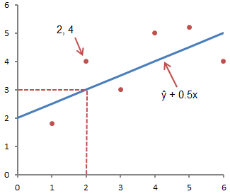
The figure below illustrates this concept graphically:
The figure above shows the line described by the equation ŷ =2+0.5x. The y-intercept is the point at which the line intersects the y-axis; in our case, a = 2. The slope of the line, b, the ratio of the rise of the line to the length of the line, has a value of 0.5. A positive slope means the line rises from left to right. If b = 0, the line is horizontal, which means there is no relationship between the dependent and independent variables. In other words, changing the value of x does not affect the value of y.
ŷ and y are often confused. The graph shows 6 ordered pairs of points and a line, according to the given equation
This figure shows the point corresponding to the ordered pair x = 2 and y = 4. Note that the expected value of y according to the line at X= 2 is ŷ. We can confirm this with the following equation:
ŷ = 2 + 0.5х =2 +0.5(2) =3.
The y value represents the actual point and the ŷ value is the expected value of y using a linear equation for a given value of x.
The next step is to determine the linear equation that best matches the set of ordered pairs, we talked about this in the previous article, where we determined the form of the equation using the least squares method.
Using Excel to Define Linear Regression
In order to use the regression analysis tool built into Excel, you must activate the add-in Analysis package. You can find it by clicking on the tab File -> Options(2007+), in the dialog box that appears OptionsExcel go to the tab Add-ons. In the field Control choose Add-onsExcel and click Go. In the window that appears, check the box next to Analysis package, click OK.
In the tab Data in a group Analysis will appear new button Data analysis.
To demonstrate how the add-in works, let's use data from a previous article, where a guy and a girl share a table in the bathroom. Enter the data from our bathroom example in Columns A and B of the blank sheet.
Go to the tab Data, in a group Analysis click Data analysis. In the window that appears Data Analysis select Regression as shown in the figure and click OK.
Set the necessary regression parameters in the window Regression as shown in the picture:
Click OK. The figure below shows the results obtained:
These results are consistent with those we obtained by doing our own calculations in the previous article.
Regression analysis is a statistical research method that allows you to show the dependence of a particular parameter on one or more independent variables. In the pre-computer era, its use was quite difficult, especially when it came to large volumes of data. Today, having learned how to build regression in Excel, you can solve complex statistical problems in just a couple of minutes. Below are specific examples from the field of economics.
Types of Regression
This concept itself was introduced into mathematics by Francis Galton in 1886. Regression happens:
- linear;
- parabolic;
- sedate;
- exponential;
- hyperbolic;
- demonstrative;
- logarithmic.
Example 1
Let's consider the problem of determining the dependence of the number of team members who quit on the average salary at 6 industrial enterprises.
Task. At six enterprises, the average monthly salary and the number of employees who quit due to at will. IN tabular form we have:
For the task of determining the dependence of the number of quitting workers on the average salary at 6 enterprises, the regression model has the form of the equation Y = a0 + a1×1 +…+аkxk, where хi are the influencing variables, ai are the regression coefficients, and k is the number of factors.
For this task, Y is the indicator of employees who quit, and the influencing factor is salary, which we denote by X.
Using the capabilities of the Excel spreadsheet processor
Regression analysis in Excel must be preceded by applying built-in functions to existing tabular data. However, for these purposes it is better to use the very useful “Analysis Pack” add-on. To activate it you need:
- from the “File” tab go to the “Options” section;
- in the window that opens, select the line “Add-ons”;
- click on the “Go” button located below, to the right of the “Management” line;
- check the box next to the name “Analysis package” and confirm your actions by clicking “Ok”.
If everything is done correctly, the required button will appear on the right side of the “Data” tab, located above the Excel worksheet.
Linear Regression in Excel
Now that you have everything you need at hand virtual instruments to carry out econometric calculations, we can begin to solve our problem. To do this:
- click on the “Data Analysis” button;
- in the window that opens, click on the “Regression” button;
- in the tab that appears, enter the range of values for Y (the number of quitting employees) and for X (their salaries);
- We confirm our actions by pressing the “Ok” button.
As a result, the program will automatically fill in a new sheet table processor regression analysis data. Pay attention! Excel allows you to manually set the location you prefer for this purpose. For example, it could be the same sheet where the Y and X values are located, or even new book, specifically designed for storing such data.
Analysis of regression results for R-squared
IN Excel data obtained during processing of the data of the example under consideration have the form:
First of all, you should pay attention to the R-squared value. It represents the coefficient of determination. IN in this example R-squared = 0.755 (75.5%), i.e., the calculated parameters of the model explain the relationship between the considered parameters by 75.5%. The higher the value of the coefficient of determination, the more suitable the selected model is for a specific task. It is considered to correctly describe the real situation when the R-square value is above 0.8. If R-squared is tcr, then the hypothesis about the insignificance of the free term of the linear equation is rejected.
In the problem under consideration for the free term, using Excel tools, it was obtained that t = 169.20903, and p = 2.89E-12, i.e., we have zero probability that the correct hypothesis about the insignificance of the free term will be rejected. For the coefficient for the unknown t=5.79405, and p=0.001158. In other words, the probability that the correct hypothesis about the insignificance of the coefficient for an unknown will be rejected is 0.12%.
Thus, it can be argued that the resulting linear regression equation is adequate.
The problem of the feasibility of purchasing a block of shares
Multiple regression in Excel is performed using the same Data Analysis tool. Let's consider a specific application problem.
The management of the NNN company must decide on the advisability of purchasing a 20% stake in MMM JSC. The cost of the package (SP) is 70 million US dollars. NNN specialists have collected data on similar transactions. It was decided to evaluate the value of the shareholding according to such parameters, expressed in millions of US dollars, as:
- accounts payable (VK);
- annual turnover volume (VO);
- accounts receivable (VD);
- cost of fixed assets (COF).
In addition, the parameter of the enterprise's wage arrears (V3 P) in thousands of US dollars is used.
Solution using Excel spreadsheet processor
First of all, you need to create a table of source data. It looks like this:
- call the “Data Analysis” window;
- select the “Regression” section;
- In the “Input interval Y” box, enter the range of values of the dependent variables from column G;
- click on the red arrow icon to the right of the “Input Range X” window and highlight on the sheet the range of all values from columns B,C,D,F.
Mark the “New worksheet” item and click “Ok”.
Obtain a regression analysis for a given problem.
Study of results and conclusions
We “collect” the regression equation from the rounded data presented above on the Excel spreadsheet:
SP = 0.103*SOF + 0.541*VO – 0.031*VK +0.405*VD +0.691*VZP – 265.844.
In a more familiar mathematical form, it can be written as:
y = 0.103*x1 + 0.541*x2 – 0.031*x3 +0.405*x4 +0.691*x5 – 265.844
Data for MMM JSC are presented in the table:
Substituting them into the regression equation, we get a figure of 64.72 million US dollars. This means that the shares of MMM JSC are not worth purchasing, since their value of 70 million US dollars is quite inflated.
As you can see, the use of the Excel spreadsheet and the regression equation made it possible to make an informed decision regarding the feasibility of a very specific transaction.
Now you know what regression is. The Excel examples discussed above will help you solve practical problems in the field of econometrics.
The linear regression method allows us to describe a straight line that best fits a series of ordered pairs (x, y). The equation for a straight line, known as the linear equation, is given below:
ŷ is the expected value of y for a given value of x,
x is the independent variable,
a is a segment on the y-axis for a straight line,
b is the slope of the straight line.
The figure below illustrates this concept graphically:
The figure above shows the line described by the equation ŷ =2+0.5x. The y-intercept is the point at which the line intersects the y-axis; in our case, a = 2. The slope of the line, b, the ratio of the rise of the line to the length of the line, has a value of 0.5. A positive slope means the line rises from left to right. If b = 0, the line is horizontal, which means there is no relationship between the dependent and independent variables. In other words, changing the value of x does not affect the value of y.
ŷ and y are often confused. The graph shows 6 ordered pairs of points and a line, according to the given equation
This figure shows the point corresponding to the ordered pair x = 2 and y = 4. Note that the expected value of y according to the line at X= 2 is ŷ. We can confirm this with the following equation:
ŷ = 2 + 0.5х =2 +0.5(2) =3.
The y value represents the actual point and the ŷ value is the expected value of y using a linear equation for a given value of x.
The next step is to determine the linear equation that best matches the set of ordered pairs, we talked about this in the previous article, where we determined the type of equation by .
Using Excel to Define Linear Regression
In order to use the regression analysis tool built into Excel, you must activate the add-in Analysis package. You can find it by clicking on the tab File -> Options(2007+), in the dialog box that appears OptionsExcel go to the tab Add-ons. In the field Control choose Add-onsExcel and click Go. In the window that appears, check the box next to Analysis package, click OK.

In the tab Data in a group Analysis a new button will appear Data analysis.

To demonstrate the work of the add-in, we will use data where a guy and a girl share a table in the bathroom. Enter the data from our bathroom example in Columns A and B of the blank sheet.
Go to the tab Data, in a group Analysis click Data analysis. In the window that appears Data Analysis select Regression as shown in the figure and click OK.

Set the necessary regression parameters in the window Regression as shown in the picture:

Click OK. The figure below shows the results obtained:

These results are consistent with those we obtained by doing our own calculations in .
CORRELATION AND REGRESSION ANALYSIS INMS EXCEL
1. Create a source data file in MS Excel (for example, table 2)
2. Construction of the correlation field
To build a correlation field in the command line, select the menu Insert/Diagram. In the dialog box that appears, select the chart type: Spot; view: Scatter plot, allowing you to compare pairs of values (Fig. 22).
Figure 22 – Selecting a chart type
Figure 23– Window view when selecting a range and rows
Figure 25 – Window view, step 4
2. In the context menu, select the command Add a trend line.
3. In the dialog box that appears, select the graph type (linear in our example) and the equation parameters, as shown in Figure 26.
Click OK. The result is presented in Figure 27.
Figure 27 – Correlation field of the dependence of labor productivity on capital-labor ratio
Similarly, we construct a correlation field for the dependence of labor productivity on the equipment shift ratio. (Figure 28).
 |
Figure 28 – Correlation field of labor productivity
on the equipment replacement rate
3. Construction of the correlation matrix.
To build a correlation matrix in the menu Service choose Data analysis.
Using a data analysis tool Regression, in addition to the results of regression statistics, analysis of variance and confidence intervals, you can obtain residuals and graphs of fitting the regression line, residuals and normal probability. To do this, you need to check access to the analysis package. In the main menu, select Service/Add-ons. Check the box Analysis package(Figure 29)
Figure 30 – Dialog box Data Analysis
After clicking OK, in the dialog box that appears, specify the input interval (in our example A2:D26), grouping (in our case by columns) and output parameters, as shown in Figure 31.
 |
Figure 31 – Dialog box Correlation
The calculation results are presented in Table 4.
Table 4 – Correlation matrix
Column 1 | Column 2 | Column 3 |
|
Column 1 | |||
Column 2 | |||
Column 3 |
SINGLE-FACTOR REGRESSION ANALYSIS
USING THE REGRESSION TOOL
To conduct a regression analysis of the dependence of labor productivity on the capital-labor ratio in the menu Service choose Data Analysis and specify the analysis tool Regression(Figure 32).
Figure 33 – Dialog box Regression